OK, from the comments I understand that the problem boils down to
$$\frac{\partial}{\partial t}\Phi_2(t,x_1,x_2)=\theta\bigl(F[\Phi_2(t,x_1,x_2)]-x_1\bigr),\;\;\Phi_2(0,x_1,x_2)=x_2,$$
where $\theta$ is the unit step function. Let me assume that $F$ is a nondecreasing function. Then the solution is
$$\Phi_2(t,x_1,x_2)=\begin{cases}
t+x_2&\text{if}\;\;F(x_2)>x_1\\
x_2&\text{if}\;\;F(x_2)\leq x_1.
\end{cases}
$$
A more general choice of $F$ can be readily accommodated, by piecing together increasing and decreasing segments. For any $F$, the function $\Phi_2(t,x_1,x_2)=x_2$ whenever $F(x_2)\leq x_1$, so we only need to consider regions in which $F(x_2)>x_1$ and $\Phi_2$ increases linearly with $t$ until $F(\Phi_2)$ becomes smaller than $x_1$.
as requested, the Mathematica code
Manipulate[Module[{sol =
             NDSolve[{phi2'[t] == UnitStep[Sin[phi2[t]] - x1], phi2[0] == x2},
                      phi2, {t, 0, tfinal}]},
             Plot[Evaluate[phi2[t] /. sol], {t, 0, tfinal}]],
                           {x1, 0, 2}, {x2, 0, 2}, {tfinal, 1, 10}]
will produce a plot of $\Phi_2(t)$ (for $F=\sin$) where you can vary $t_{\rm final}$, $x_1$, and $x_2$.
alternatively, the Mathematica code
sol = NDSolve[{D[phi2[t, x1, x2], t] ==
               UnitStep[Sin[phi2[t, x1, x2]] - x1], phi2[0, x1, x2] == x2}, phi2,
               {t, 0, 5}, {x1, 0, 2}, {x2, 0, 2}];
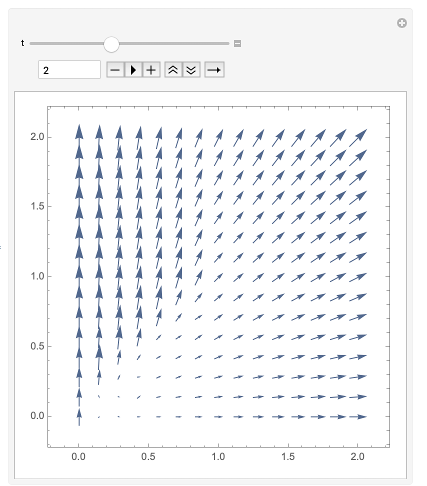
 Manipulate[VectorPlot[{x1, Evaluate[phi2[t, x1, x2] /. sol]},
               {x1, 0, 2}, {x2, 0, 2}], {t, 0, 5}]
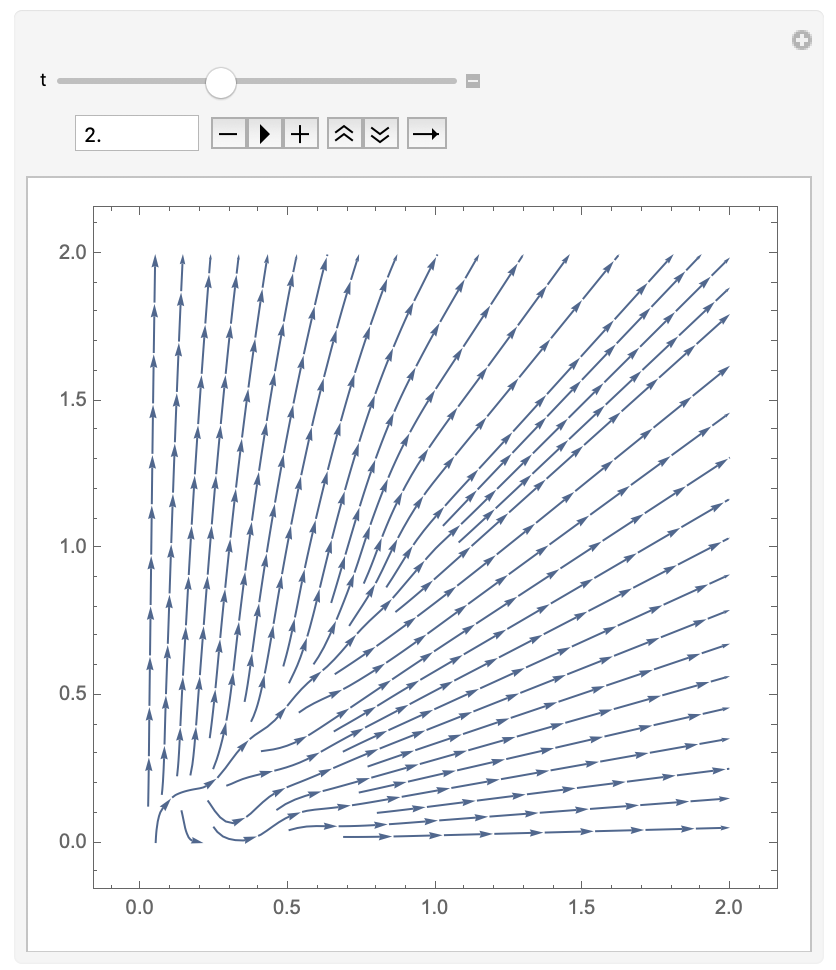
 Manipulate[StreamPlot[{x1, Evaluate[phi2[t, x1, x2] /. sol]},
               {x1, 0, 2}, {x2, 0, 2}], {t, 0, 5}]
will produce a vector plot or a stream plot of $(\Phi_1,\Phi_2)$ in the $x$-$y$ plane, with $t$ as a parameter that you can vary.


