Time of peak of an SIR epidemic

Question

I've learned some classical results on the peak and the attack rate of an idealized epidemic which evolves according to a SIR model

• $\dot{s} = -\beta\cdot i \cdot s$
• $\dot{i} = +\beta\cdot i \cdot s - i/\delta$
• $\dot{r} = +i/\delta$

with infection rate $\beta$ and duration of infectiosity $\delta$, the basic reproduction number being $R_0 = \beta \cdot \delta$.

The classical results I have learned:

For $s(0) \approx 1$ the maximum of $i(t)$ is given by

$$i_{max} = \frac{R_0 - \ln{R_0} - 1}{R_0}$$

(see e.g. Hethcote's The Mathematics of Infectious Diseases, Theorem 2.1, p. 607)

and the attack rate $r_\infty = \lim_{t\rightarrow \infty}r(t)$ is given by

$$r_\infty = 1 + \frac{W(-R_0 e ^{-R_0})}{R_0}$$

with the Lambert W function (see e.g. here, Proposition 1.10, p. 3)

What I still haven't found is a reference for the time $t_{max}$ at which $i(t)$ reaches its maximum (i.e. $i(t_{max}) = i_{max}$) when $i(0) = i_0$ is given and $r(0) = 0$.

Find here some plots with a single patient 0 in a completely susceptible population of 10,000, i.e. $i_0 = 0.0001$. A period of 90 days is displayed. $[\delta] =$ 1 day, $[\beta] = $ 1/day.

The peaks for $\beta_1\delta_1 = \beta_2\delta_2$ – for example $[4,1.5]$ and $[6,1]$ or $[2,1.5]$ and $[4,0.75]$ or $[2,1]$ and $[4,0.5]$ – have the same $R_0 = \beta\delta$ and thus roughly⁽¹⁾ the same $i_{max}$, but they differ in $t_{max}$. So even though $t_{max}$ decreases with increasing $R_0$ for fixed $\beta$ or $\delta$ (which is quite natural), it cannot depend on the product $\beta\delta$ alone (as $i_{max}$ does) but must depend also on the quotient $\beta/\delta$ or maybe the difference $\beta - 1/\delta$. _{(1) Roughly because of errors due to finite time steps $\Delta t$ instead of infinitesimal $dt$.}

To get a better picture of the heights and timings of the peaks, these are all the curves above overlayed:

A good algebraic approximation for $t_{max}$ as a function of $\beta$ and $\delta$ would be welcome (assuming that no closed formula exists) – or simply a reference. (Consider $i_0$ a fixed parameter and $r(0) = 0$.)

Note that $\beta/\delta$ has a unit of 1/day² and thus of an acceleration.

Answer 1

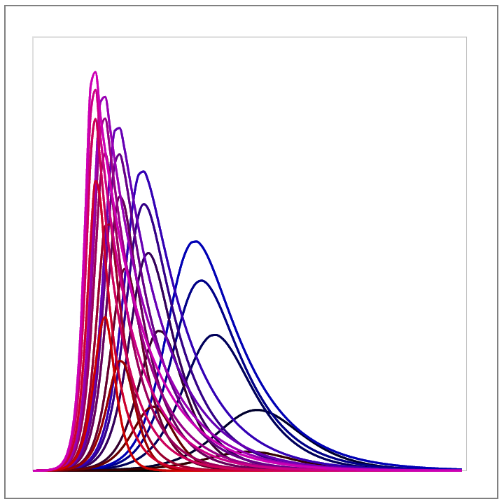
Seems like you fell in love with those equations and, especially, with the $I$ component of them:-). So let me try to show you how you can derive as many approximations as you want yourself, test them against simulations and (if you are lucky) find a few to your liking. Again, I'll put everything in the numerator: $\dot S=-\beta IS, \dot E=\beta IS-\lambda E, \dot I=\lambda E-\delta I, \dot R=\delta I$. I'll also normalize to $\lambda+\delta=1$ (time scaling) and denote $\rho=\lambda\delta\in(0,\frac 14]$ after such normalization. The total population will be normalized to $1$.

We shall assume that we are in the situation when the initially infected and exposed portions are very small and everyone is susceptible Note that for a while (when $S\approx 1$), you run just a linear system on $I$ and $E$. Anything can happen here: for instance, if $E=0$, then $I$ initially goes down and there is no way its graph can match your idea of a peaking curve on that interval. We want to eliminate the decaying part of the solution from the initial data.

Fortunately, the linear theory is easy: you expect that all growth is determined by the eigenvector corresponding to the largest eigenvalue. The eigenvalues for the EI part are (under my normalization) $-0.5\pm\sqrt{0.25+(\beta-\delta)\lambda}$. So, you decompose the vector $(E,I)$ into the parts proportional to the eigenvectors and take the $I$-component of the part corresponding to the positive eigenvalie. That is your $I_{eff}$. You can now presume that starting with $I_{eff}$ and $E_{eff}$, you can run your approximate curve, whatever you decide it to be, infinite time in both directions. Thus, if you settled on some analytic curve $I(t)=F(t)$ approximating your solution that has the maximum at the origin and satisfies the equation on the whole line, then you just solve the equation $F(-t_{max})=I_{eff}$. Now about how to find decent curves that describe the pandemic coming from $-\infty$ with $S=1,I=E=R=0$ there and going to $+\infty$ with $I=E=0$ there. First of all, determine the quantities that you know exactly. There is actually just one such quantity: the full integral $J=\int_{-\infty}^\infty I(t)dt$. It has two meanings. On one hand, $\delta J=R(+\infty)$. On the other hand, $e^{-\beta J}=S(+\infty)$. Then we get our first equation: $$ e^{-\beta J}+\delta J=1, $$ which can be solved in a unique way for $J>0$. So, from now on, I'll treat $J$ as a known quantity available for using in other formulae.

Next, generally speaking, we need to decide on some parametric family of curves $F_p(t)$, where $p$ is a set of parameters, that can be used for curve fitting. We need at least 2 free parameters since, after my normalization, we have $2$ degrees of freedom in the choice of $\beta,\lambda,\delta$. However, having just 2 formal parameters from the start seems too restrictive because we then need to guess everything just right. On the other hand, introducing too many parameters is also bad because we shall get too many complicated equations. So, perhaps, three or four would be a good choice. Note that we already have one nice to use relation for $p$: $$ \int_{-\infty}^{\infty}F_p(t)\,dt=J\,. $$ so ideally this integral should be at least approximately computable in terms of $p$.

Let's see what else we can discern before deciding on any particular kind of curve. Write $I=\frac{I_0}{\psi}$ where $I_0$ is the maximal value attained at $0$. Then we can successively express $E$ and $S$ in terms of $\psi$ and its derivatives. This algebraic exercise yields $$ \lambda E=\delta I+\dot I=I_0\left[\frac \delta\psi-\frac{\dot\psi}{\psi^2}\right] \\ \beta\lambda SI=\lambda \dot E+\lambda(\lambda E)=I_0\left[\frac\rho\psi-\frac{\dot\psi}{\psi^2}-\frac{\ddot\psi}{\psi^2}+2\frac{\dot\psi^2}{\psi^3}\right] \\ \beta\lambda S=\rho-\frac{\dot\psi}{\psi}-\frac{\ddot\psi}{\psi}+2\frac{\dot\psi^2}{\psi^2} $$ (I used the normalization $\lambda+\delta=1$ in the process). Now denote $B=\beta I_0$. The last equation that we haven't used (that for $S$) reads in this notation $$ -\dddot\psi-\ddot\psi+5\frac{\dot\psi\ddot\psi}{\psi}-4\frac{\dot\psi^3}{\psi^2}= -B\left[\rho-\frac{\dot\psi}{\psi}-\frac{\ddot\psi}{\psi}+2\frac{\dot\psi^2}{\psi^2} \right]\,, $$ which looks a bit scary until you realize that for every exponent $a\in \mathbb R$ (with one exception, which I leave to you to find), it has an asymptotic solution $ce^at+b+\dots$ at each infinity (the exponent is presumed to grow at the infinity here and $\dots$ stand for the decaying terms). To see it, just plug this form into the equation and find $b$ that eliminates all growth and constants (it depends on $a$, of course). Now, it seems a good idea to presume that our actual solution of the IVP $\psi(0)=1,\dot\psi(0)=0$ also has this asymptotic form. Moreover, from the expression for $\beta\lambda S$, which can be rewritten as
$$ \rho-\frac{\dot\psi}{\psi}-\frac{d}{dt}\frac{\dot\psi}{\psi}+\frac{\dot\psi^2}{\psi^2} $$ we can immediately see the equations for the exponents. Indeed, if $\psi\asymp e^{at}$, then $\frac{\dot\psi}{\psi}\to a$ and the derivative of it goes to $0$, so at $\pm\infty$, we have for the corresponding exponents $$ \delta-a_{\pm}+a_{\pm}^2=\beta\lambda S(\pm\infty) $$ and we know that $S(-\infty)=1$, $S(+\infty)=e^{-\beta J}$. So, these quadratic equations allow us to find $a_-$ as the unique negative root $0.5-\sqrt{0.25+(\beta-\delta)\lambda}$, which not surprisingly is just minus the "onset exponent" we found earlier. For $a_+$ we have two choices but it turns out that it is the smaller root that we really need (both are positive). Thus, our $F_p$ should be asymptotic to $e^{a_\pm t}$ at infinities at least approximately, which gives us two more equations for $p$. Finally, it would be nice to have our ODE satisfied at least at the point of the maximum to have the local behaviour near $0$ not too weird. This is the fourth equation. Thus, we should have at least 4 parameters not to sacrifice anything. We already have one: $I_0$, or, which is the same, $B$. It seems rather natural to take the two exponents $a_{\pm}$ as the other two, especially because we can force their values to be exactly right without much trouble. Thus, we need one more.

Here you have options. I played with a few and finally settled on the function of the kind $$ \psi(t)=c+c_+e^{a_+t}+c_-{ea_-t} $$ where $c\in[0,1)$ and $c_\pm$ can be immediately determined from $c$ and the conditions $\psi(0)=1,\dot\psi(0)=0$. The differential equation at the point $0$ of maximum becomes then a nice algebraic relation between $c$ and $B$ (quadratic, to be exact) once $a_{\pm}$ are known.

The nightmare equation then becomes the very first one: $\int F_p=J$. This requires to integrate $\frac 1{\psi}$ and there is no nice formula. However, there is a nice approximation: when $c=0$, we can find the full integral using residue technique, and when $a_-=-a_+$, we can find the dependence of $c$ exactly, so we just assume that it expands to the other values approximately. The quick numeric check shows that this assumption is not as idiotic as one can think, so we get the final relation, which, if you put everything together, reads $$ B\frac{2}{\sin(\pi t)t^t(1-t)^{1-t}} \frac 1{a_+-a_-}\frac {\arctan(\frac{\sqrt{1-2c}}c)}{\sqrt{1-2c}}=\beta J $$ where $t=a_+/(a_+-a_-)$ (or something like that: when $c>\frac 12$, you need to replace the arctangent by the difference of logarithms: it is the same analytic function but the algebra is not programming-friendly here). Of course, you are more than welcome to experiment with other forms of the solutions.

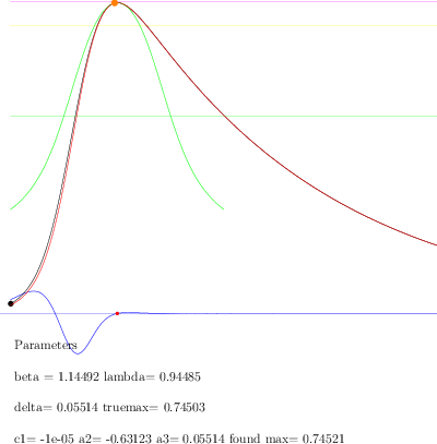
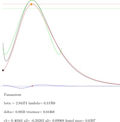
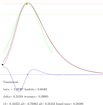
Now, once you solve the resulting system, you can plug everythin in and see if the curve matches the simulation. Here are a few pictures: the black curve is the numeric solution of the ODE, the red curve is the fitting one (of the above kind), the green one is the best symmetric approximation, the blue line is the error in the equation (scaled in some reasonable way), the orange dot is the predicted time of maximum, the magenta horizontal line is the predicted maximum, etc.

Can one learn anything from this exercise? Honestly, I have no idea. I just wanted to show you how such things can be done, so you can try yourself. The approximate parametric form I suggested here is quite simple, but determining the parameters from $\beta,\lambda,\delta$ requires solving a few transcendental equations. The fit is pretty good though up to $\frac{\beta}{\delta}\approx 20$ uniformly in $\lambda$.