$L^p$-convergence of truncated Legendre series approximation to inverse error function $\text{erfinv}$

Question

Bounding the $L^p$-error for an $n$-th order Legendre series approximation

I have function $f\,\colon (-1, 1) \to \mathbb{R}$ where $f \in L^q(-1, 1)$ for any $q \geq 1$. I approximate $f$ using a truncated Legendre series $g_n $ up to the $n$-th order polynomial term. As this is the Legendre series this is the best approximation as measured by the $L^2$-error for an $n$-th degree polynomial. I would like to find the convergence rate of the $L^p$-error for any $p \geq 2$ as $n\to\infty$. Given $f \in L^q(-1, 1)$ for any $q \geq 1$ I expect this is a standard result to people more familiar with approximation theory than myself, but I am struggling to find a source with the solution.

\begin{equation} ||f - g_n||_{L^p(-1,1)} < \quad \text{???} \end{equation}

Empirical results

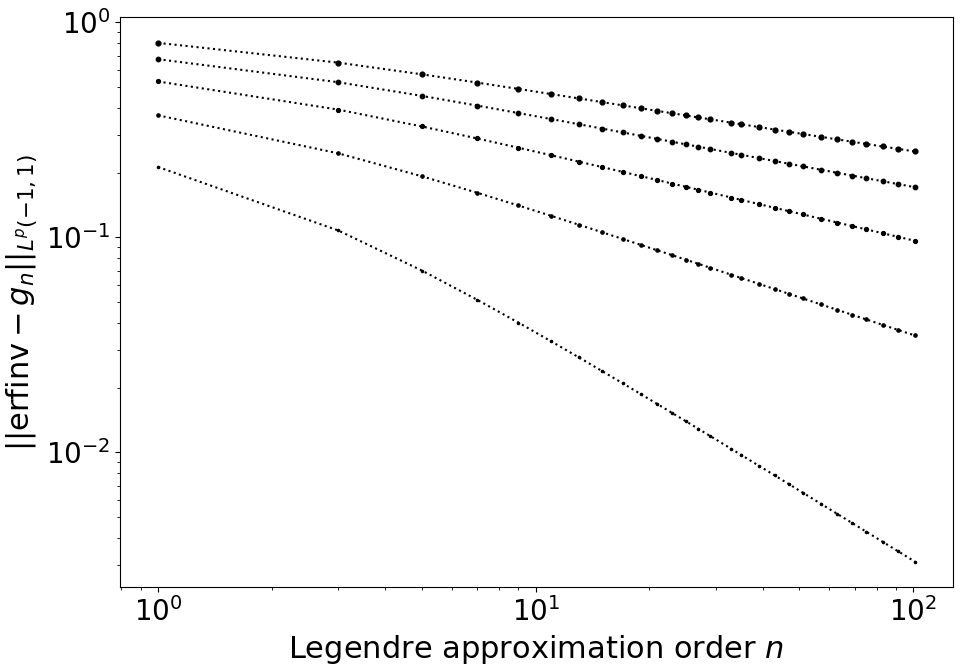
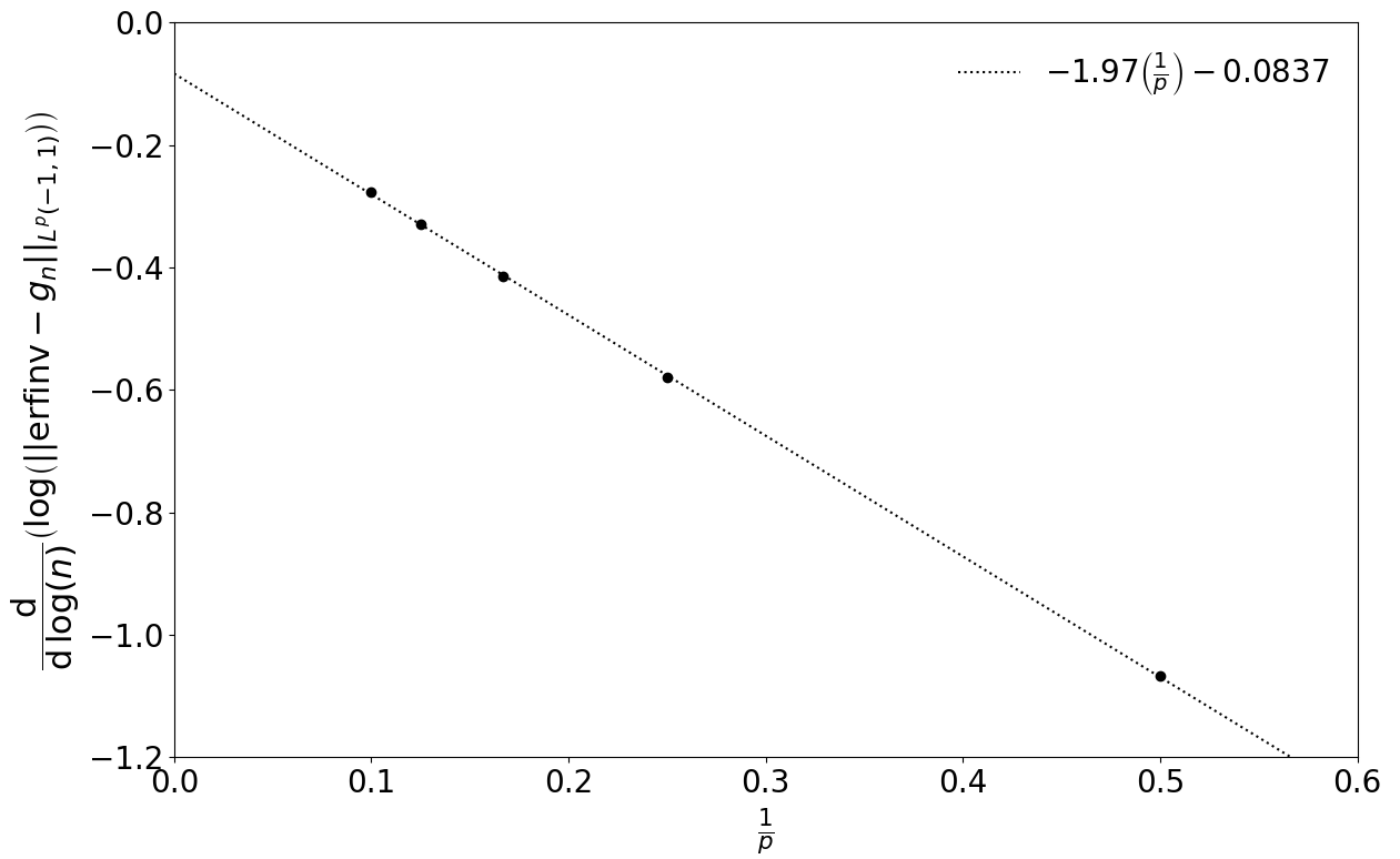
The specific function I am interested in is the inverse Gaussian CDF $\Phi^{-1}(\cdot)$, for which it is sufficient to consider the inverse error function $\text{erfinv}(\cdot)$ because $\Phi^{-1}(x) = \sqrt{2}\,\text{erfinv}(2x-1)$ for $x \in (0, 1)$. Doing the numerics for this I find empirically \begin{equation} ||\text{erfinv} - g_n||_{L^p(-1,1)} < C n^{-0.08 - 2/p}, \end{equation} where I have considered polynomials up to order 500.

For inverse error function we know $\text{erfinv} \in L^q(-1, 1)$ for any $q \geq 1$ because if we change the integral expression of the $L^q$-norm it corresponds to the moments of the standard normal, which for any finite moment $q$ are all finite.

Some results similar to what I'm after

Results from spectral methods

Based on this answer to Polynomial approximation in L^p norms it has lead me to Spectral Methods: Fundamentals in Single Domains by Canuto et al. I'm away from my department library and so only have limited access to some google pages, and several of the results on the truncated Legendre series errors aren't shown. A closer/reminiscent result is (5.5.10) on page 293, but this uses Chebyshev series $P_n$:

\begin{equation} ||f-P_n||_{L^p_w(-1, 1)} \leq C n^{-m} \sum_{k=\min\{m, n+1\}}^m ||f^{(k)}||_{L^p_w(-1, 1)} \qquad (5.5.10) \end{equation}

Work by Harry Pollard

In the works by Pollard there are two related results. The first is from The mean convergence of orthogonal series I (1947), where the main results is that $p$-mean convergence only holds for $\tfrac{4}{3} < p < 4$ and fails for $p > 4$. This seems to pivot on the Legendre series failing to form a basis for $p > 4$ and centres on his result:

Theorem 8.1: The Legendre polynomials form a basis for $L^p(-1, 1)$ if $\tfrac{4}{3} < p < 4$.

This result was extended in Mean convergence of orthogonal series (1952) by Newman and Rudin to cases $p=\tfrac{4}{3}$ and $p = 4$.

There is a later result by Pollard in The Convergence Almost Everywhere of Legendre Series (1972):

Theorem. If $f \in L^p$ for some $p$ in the range $\tfrac{4}{3} <p < \infty$, then its Legendre series converges p.p.

With both these works by pollard, neither give a rate of convergence, and looking through the work one doesn't seem to crop up. Furthermore, my numerics for the inverse error function seem to suggest there is $p$-mean convergence for $p \geq 4$, unlike the theory from the paper.

The numerics

Computing the $L^p$-error for $p \in \{2,4,6,8,10\}$

Performing a linear regression for $n\geq 10$ where the log-log plot becomes linear.

Code

import matplotlib.pylab as plt
import numpy as np
from mpmath import mp
from sklearn.linear_model import LinearRegression
mp.dps = 20

from functools import wraps


def memoize(function):
    cache = {}

    @wraps(function)
    def wrapper(*args):
        if args in cache:
            return cache[args]
        else:
            val = function(*args)
            cache[args] = val
            return val

    return wrapper

### The coefficients for the L2 fitting ###
cdf = mp.ncdf
pdf = mp.npdf
sqrt = mp.sqrt
pi = mp.pi
fabs = mp.fabs
inf = mp.inf
log10 = mp.log10
log = mp.log
erfinv = mp.erfinv
legendre = lambda n, x: mp.legendre(n, x)
x = mp.fabs(1.0) * np.linspace(-1, 1, 1000)[1:-1]
u = (x + 1.0) / 2.0
e = [erfinv(i) for i in x]
ze = [ppf(i) for i in u]


@memoize
def get_n_th_order_legendre_coeff(func, n):
    return (n + 0.5) * mp.quad(lambda x: func(x) * legendre(n, x), [-1, 1], method='tanh-sinh')


def construct_l2_legendre_approximation_odd_function(func, max_order):
    """
    Constructs the Legendre series approximation of an odd function.
    :param func: Function with domain [-1, 1].
    :param max_order: Int.
    :return: Function.
    """
    orders = range(1, max_order + 1, 2)
    coeffs = [get_n_th_order_legendre_coeff(func, n) for n in orders]

    def legendre_approximation(x, order):
        return sum([coeff * legendre(n, x) for coeff, n in zip(coeffs, orders) if n <= order])

    return legendre_approximation


max_order = 300
erfinv_legendre_approx = construct_l2_legendre_approximation_odd_function(erfinv, max_order)


def round_up_to_odd(f):
    return np.ceil(f) // 2 * 2 + 1


# Getting some roughly evenly spaced points in log-space.
orders = list(sorted({int(round_up_to_odd(int(i))) for i in np.logspace(0, np.log10(100), 50)}))
p = [2, 4, 6, 8, 10]  # p = 1 is invalid
l_p = {i: [] for i in p}
for order in orders:
    print('Working on order {}'.format(order))
    for p in l_p.iterkeys():
        l_p[p].append(mp.quad(lambda x: (erfinv_legendre_approx(x, order) - erfinv(x)) ** p, [-1, 1], method='tanh-sinh') ** (1.0 / p))

plt.clf()
for p in l_p.iterkeys():
    plt.plot(orders, l_p[p], 'ko:', ms=np.log2(1 + p))
# plt.plot(orders, orders, 'ro')
plt.yscale('log')
plt.xscale('log')
plt.xlabel('Legendre approximation order $n$')
plt.ylabel(r'$||{\rm erfinv} - g_n||_{L^p(-1, 1)}$')

l_p_t = {p: a[5:] for p, a in l_p.iteritems()}  # Truncating the points we fit to.
lxy = {p: [np.log(np.float64(orders[-len(a):])), np.log(np.float64(a))] for p, a in l_p_t.iteritems()}
lxy = {p: LinearRegression().fit(xy[0].reshape(-1, 1), xy[1]).coef_[0] for p, xy in lxy.iteritems()}
p, c = zip(*lxy.iteritems())
p, c = [np.array(i)[np.argsort(p)] for i in [p, c]]
plt.clf()
plt.plot(1.0 / p, c, 'ko')
reg = LinearRegression().fit((1.0 / p).reshape(-1, 1), c)
x = np.linspace(0, 0.6, 1000)
y = reg.intercept_ + reg.coef_ * x
plt.plot(x, y, 'k:', label=r'$-1.97\left(\frac{1}{p}\right) - 0.0837$')
plt.legend(frameon=False)
plt.xlim(0, 0.6)
plt.ylim(-1.2, 0)
plt.xlabel(r'$\frac{1}{p}$')
plt.ylabel(r'$\dfrac{\mathrm{d}}{\mathrm{d}\,\log(n)} \left(\log\left(||{\rm erfinv} - g_n||_{L^p(-1, 1)}\right)\right)$')