Here $\{\cdot\}$ and $\lfloor \cdot\rfloor$ denote the fractional part and floor functions respectively. For a negative, non-integer number $x$, we use the following definition: $\{x\}=1-\{-x\}$. If $x$ is a negative integer, $\{x\} =0$. We are dealing with the following recurrence:
$$X_{k+2}=\{b_2 X_{k+1}+b_1 X_k\}$$
where $X_1$ is a uniform random variable on $[0,1]$ and $X_0\in [0,1]$ is a constant. Thus all the $X_k$'s are in $[0,1]$. Also, $b_1, b_2$ are integers, called bases; they represent bases in a numeration system.
The simple case: $b_1=0$
I extensively studied the case $b_1=0, b_2 > 1$ corresponding to a first-order recurrence, see here. The main results are:
The sequence $\lfloor b_2X_k \rfloor$ corresponds to the digits of $X_1$ in base $b_2$. These digits behave as independently and identically distributed discrete uniform variables on $\{0, 1,\cdots,b-1\}$.
The sequence $X_k$ behaves as identically distributed continuous uniform variables on $[0, 1]$. The correlation between $X_k$ and $X_{k+m}$ is equal to $b_2^{-m}$.
For a specific value of $X_1$, say $X_1=c$ with $c$ a normal number (say $c=\log 2$), the empirical process of observed $X_k$'s (corresponding to a specific realization of the theoretical stochastic process) satisfies the same properties for the empirical statistics: convergence of the empirical distribution to uniform on $[0, 1]$, convergence of the empirical auto-correlations to the theoretical values mentioned above, etc.
This happens because the sequence is ergodic. Note that almost all numbers are normal, though no one knows if any of $e,\pi,\sqrt{2},\log 2$ is normal. They are believed to be normal.
The general case, and my question
The general case is when both $b_1$ and $b_2$ are non zero. For simplicity, we can focus on the following specific case, which seems to behave very nicely: $X_0=\frac{1}{2}, b_1=-3, b_2 = -5$. More specifically, it now looks like the $X_k$'s are not only uniformly distributed on $[0, 1]$, but also asymptotically independently distributed. Thus we can use that sequence as a random number generator, with $X_1$ being the seed. This is a big contrast with the simple case discussed in the first section.
For instance (this is an illustration of what I mean by asymptotic independence), if $X_1=\frac{\sqrt{2}}{2}$, the empirical probabilities satisfy
$$\hat{P}\Big[\bigcap_{i=0}^m (X_{k+i}<\alpha_i)\Big]\rightarrow \prod_{i=0}^m \hat{P}\Big[X_{k+i}<\alpha_i\Big]\rightarrow\prod_{i=0}^m \alpha_i$$
regardless of $m$ and $0\leq \alpha_0,\cdots,\alpha_m\leq 1$, when more and more terms (that is more and more $k$'s) are used to estimate these probabilities. I thus assume (maybe erroneously) that it must also be true for the theoretical properties. This is illustrated further in the Appendix (last section).
My question is whether my conjecture (independence of the $X_k$'s) is true. It was verified empirically when $X_0=\frac{1}{2}, X_1=\frac{\sqrt{2}}{2}, b_1=-3, b_2=-5$, as well as for many other parameter sets. The generated deviates seem to approach randomness better than those generated using Excel, based on various statistical tests. Note that not any parameter set works; there are plenty of exceptions, and identifying these exceptions would be a bonus.
Computational considerations
No need to read this section, only if you are interested, but it is not directly related to my question.
When you compute the successive $X_k$'s, you lose one bit of precision at each iteration. This is not an issue thanks to ergodicity, it's like re-starting the sequence with new seeds every 45 or so iterations. It's only an issue if you look e.g. at long-range auto-correlations.
Also, it is possible to carry the computations very efficiently. You start with getting and storing several billions of binary digits of $X_1=\frac{\sqrt{2}}{2}$. See here how you can get these digits. Then you only need to perform simple additions and bit shifting with a big number library. For instance, $5x = 4x + x$, and computing $4x$ is just a bit shifting operation (no multiplication involved). Likewise with $3x=2x + x$. In my Perl code, if I use this little trick, it runs 10 times faster than doing an actual multiplication.
Appendix
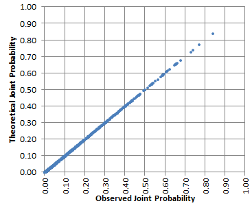
I estimated the probability $P(X_k<\alpha_0, X_{k+1}<\alpha_1, X_{k+2}<\alpha_2)$ for a thousand randomly selected triplets $(\alpha_0,\alpha_1,\alpha_2)$ in $[0, 1]^3$ and 100,000 $(X_k,X_{k+1},X_{k+2})$'s. Assuming uniform distribution and independence between $X_k, X_{k+1}$ and $X_{k+2}$, the theoretical value is always $\alpha_0\cdot \alpha_1\cdot \alpha_2$. The data and source code is available in an Excel spreadsheet, here. It is very easy to replicate my results. The observed and theoretical values are extremely close, supporting the conjecture of stochastic independence and uniformity. Below is a scatter plot where each point corresponds to one of the $(\alpha_0, \alpha_1, \alpha_2)$'s, with the X-axis being the observed (estimated) probability, and the Y-axis being the theoretical probability (the product of $\alpha_0,\alpha_1,\alpha2$).
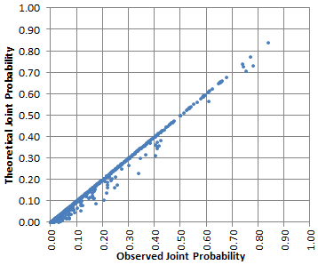
By contrast, here is an example where the independence assumption is violated, corresponding to $b_1=0, b_2=3$ with $\mbox{Correl}(X_k,X_{k+1}) = \frac{1}{3}$ and $\mbox{Correl}(X_k,X_{k+2}) = \frac{1}{9}$:
In short, in the example with independence (first chart) you seem to have, assuming $X_1$ is uniformly distributed on $[0,1]$: $$P(X_{k+2}\in A_2 | X_{k+1}\in A_1, X_k\in A_0)=\mu(A_2)$$ where $A_0, A_1, A_2$ are Borel subsets of $[0, 1]$ and $\mu(\cdot)$ is the Lebesgue measure. Yet it is obviously true that $X_{k+2}-b_2X_{k+1}-b_1X_k$ can only take on $|b_1|+|b_2|$ distinct integer values. Note that if you consider the sequence $Y_k=X_{3k}$ instead, then the triplets $(Y_k,Y_{k+1},Y_{k+2})$ don't lie in a small number of planes, unlike the $X_k$'s.


