A problem on real valued functions in $\mathbb{R}^2$ with least variation

Question

Let $\alpha(s) = (x(s),y(s))$ be the arc length parametrization of a plane, smooth, closed, convex curve, of length $L$. Let $J:(0,L)\to\mathbb{R}$ be a smooth and Bounded variation (BV introduced after comment from Dirk of possibility of blow up at 0 or L) function. Let $\Omega$ be the set of all interior points of the region bounded by the curve $\alpha(s)$.

The problem I would need help for, is to determine $f:\Omega \to \mathbb{R}$, such that

1. Given any $s_0 \in (0,L)$, and let $p_0 = \alpha(s_0)$, $${\lim_{p\to p_0}}_{p\in\Omega}f(p) = J(s_0)$$

2. $f\in C^{\infty}(\Omega \setminus R)$, where $R$ is a set of 1-Hausdorff measure equal to 0.

3. The total variation $V(f,\Omega)$ is minimum possible.

Motivation : Trying to define step functions in $\mathbb{R}^2$

PS :

^ Picture source : Wikipedia

Answer 1

You want to solve this problem $$ \min \{V(f,\Omega)\ : f\in BV(\Omega),\ f|_{\partial \Omega}\equiv J \} $$ and there is quite some background required to analyze this problem.

First, one should clarify existence of solutions, then uniqueness, then one could also think about regularity of solutions and finally, analytical or numerical methods.

First, you should look for solutions $f$ in the space $BV(\Omega)$ and not in $C^\infty(\Omega)$ (it may well be, that there is a solution that has additional regularity, but that's a question for a later stage). This may feel like making the problem more complicated than it is, but in fact the framework of $BV$-functions is indeed quite flexible and somehow, only $BV$ reveals what is really going on here.

Then one would clarify in what sense a function $f\in BV(\Omega)$ has boundary values. In fact, there is a well defined trace operator taking $f\in BV(\Omega)$ to $f|_{\partial\Omega}\in L^1(\partial\Omega)$ (cf. Theorem 10.2.2 from "Variational Analysis in Sobolev ans BV spaces" by Attouch et al.). Then existence of solutions is clear from standard arguments along the lines of what is called "the direct method in the calculus of variations" (you know, minimizing sequences, weak cluster points, lower semi-continuity and so on).

I should not that the problem you want solve is pretty famous in mathematical image processing and know as inpainting: You have some image $u_0$ defined on some domain $D\setminus\Omega$ (i.e. some domain $D$ and the part inside $\Omega$ is missing). You want to fill in the image $u_0$ in some meaningful way. One idea (and not the best) is to look for some $u$ defined on all of $D$ such that $u$ is equal to $u_0$ outside of $\Omega$ and has minimal total variation in $\Omega$ (that's equal to your problem with boundary values).

A point to get started about algorithms is the IPOL-Article by Pascal Getreuer Total Variation Inpainting using Split Bregman. There you'll find code for a numerical solution and also some pointers to relevant literature.

Regarding regularity of solutions (e.g. smooth solutions for smooth boundary values along a smooth curve), I am not sure and this may be difficult.

I suspect that solutions may not be unique and that there are situations in which there are both smooth and nonsmooth solutions. Indeed in the one dimensional case there are multiple solutions for the boundary values $f(0)=0$ and $f(1)=1$: all increasing functions with these boundary values have total variation equal to one which is minimal. Note that there are smooth solutions but also nonsmooth ones (even ones that jump). It is not clear to me, if the situation in higher dimensions could be any better…

Answer 2

I roughly sketch a solution without a proof, and also a possible minimum possible value for total variation of $f$.

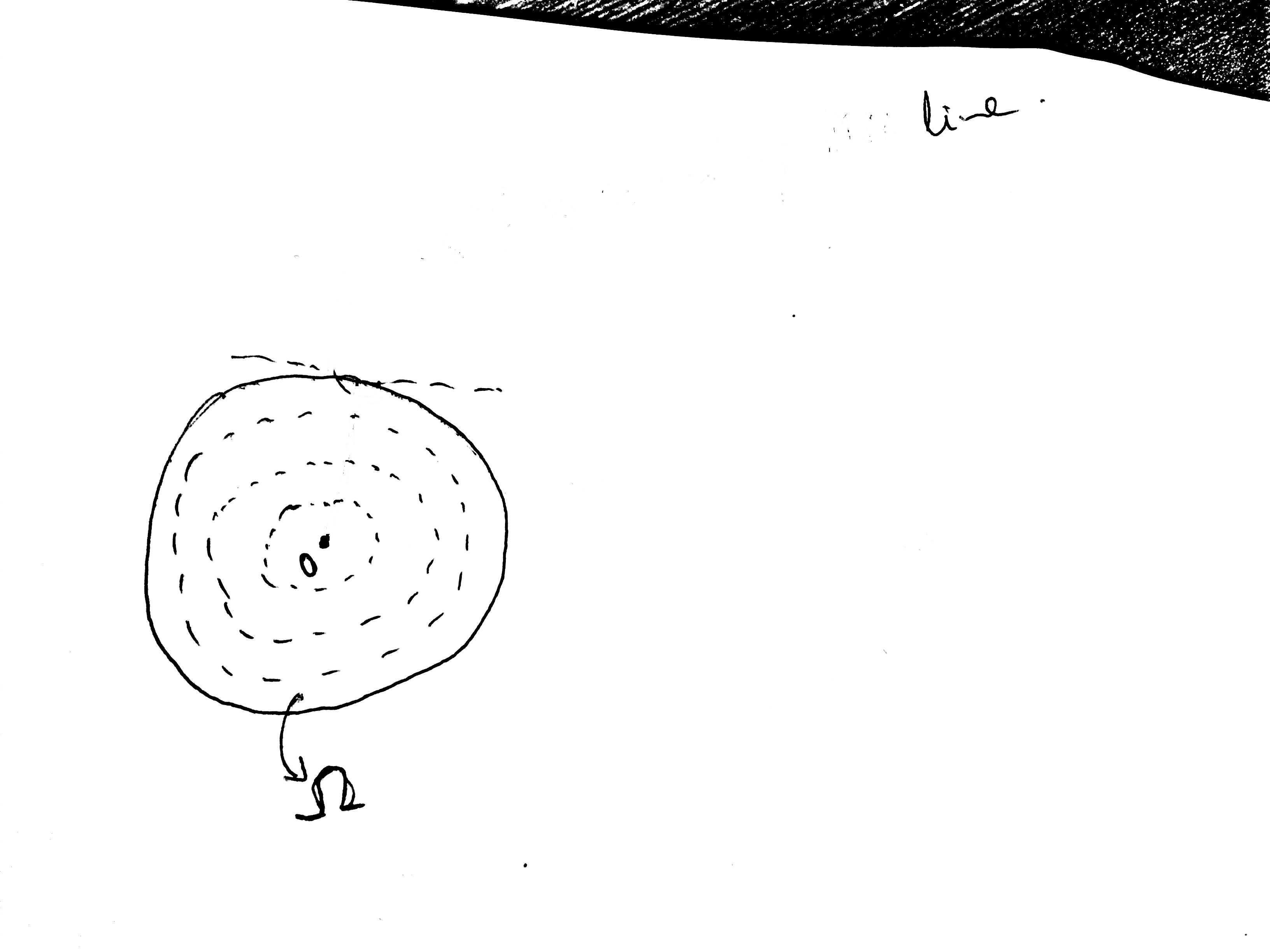
Let $f$ assume values of $J$ on the boundary curve $\alpha$. We construct infinite number of scaled down versions of the curve $\alpha$ with scale factor ranging from $1$ and converging to $0$, and on each curve we let $f$ take values of corresponding scaled down version of $J$.

Edit : (clarify) If curve is scaled by $c$, then new $J_c(x) = J(\frac{x}{c})$, where $J_c$ is defined on $(0,Lc)$. $c\in(0,1)$

This is illustrated roughly in the picture below.

This way we construct $f$ on entire $\Omega$ and it is smooth(as $J$ and $\alpha$ are smooth) except possibly at $O$, the centroid of region $\Omega$, where it is not continuous. But this discontinuty at $O$ has no effect on Variation of $f$ in $\Omega$.

Variation of $f$ for this case, is given as $$V(f,\Omega) = V_0^L(J) \mathcal{H}^2(\Omega)$$

I am yet to sketch a proof that this is the minimum possible variation for $f$.

PS : $V_0^L(J)$ is the total variation of $J$ in $(0,L)$, and $\mathcal{H}^2(\Omega)$ is the two dimensional Hausdorff measure of the set $\Omega$.