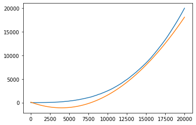
It turns out the story for $m>2$ permutations is virtually identical to the story for $2$ permutations. Furthermore, using linearity of expectation, we can greatly simplify our calculations.
Fix $m\geq{2}$ and suppose that $\sigma_{1}, \sigma_{2}, ..., \sigma_{m}$ are i.i.d. permutations, sampled uniformly at random from $S_{n}$. Define the random function $f_{n}:\{1,2,3, ..., n\}\rightarrow{\{0, 1, 2, ..., n\}}$ as follows:
$$
f_{n}(k)=|\cap_{i=1}^{m}\sigma_{i}(\{1,2,3,....,k\})|
$$
By linearity of expectation,
\begin{align*}
\mathbb{E}\big(f_{n}(k)\big)&=\mathbb{E}\big(\sum_{j=1}^{n}1_{(j\in{\sigma_{i}(\{1,2,3,...,k\})} \hspace{2pt}\text{for all}\hspace{2pt} i )}\big)=\sum_{j=1}^{n}\mathbb{E}\Big(\prod_{i=1}^{m}1_{(j\in{\sigma_{i}(\{1,2,3,...,k\}))}}\Big) \\
&=\sum_{j=1}^{n}(\mathbb{E}1_{(j\in{\sigma_{1}(\{1,2,3,...,k\}))}})^{m}=n\big(\mathbb{P}(1\in{\sigma_{1}(\{1,2,3,...,k\})})\big)^{m} \\
&=n\left(\frac{\binom{n-1}{k-1}}{\binom{n}{k}}\right)^{m}=n\left(\frac{k}{n}\right)^{m}
\end{align*}
Similarly, we can compute the second moment:
\begin{align*}
\mathbb{E}\big(f_{n}(k)\big)^{2}&=\mathbb{E}\big(\sum_{j=1}^{n}1_{(j\in{\sigma_{i}(\{1,2,3,...,k\})} \hspace{2pt}\text{for all}\hspace{2pt} i )}\big)^{2} \\ &=\mathbb{E}\big(\sum_{j=1}^{n}1_{(j\in{\sigma_{i}(\{1,2,3,...,k\})} \hspace{2pt}\text{for all}\hspace{2pt} i )}\big)+2\mathbb{E}\big(\sum_{1\leq{j_{1}}<j_{2}\leq{n}}1_{(j_{1}, j_{2}\in{\sigma_{i}(\{1,2,3,...,k\})} \hspace{2pt}\text{for all}\hspace{2pt} i )}\big) \\
&= n\left(\frac{k}{n}\right)^{m} + 2\cdot{\frac{n(n-1)}{2}}\cdot\mathbb{P}\big(1,2\in{\sigma_{1}(\{1,2,...,k\})}\big) \\
&= n\left(\frac{k}{n}\right)^{m} + n(n-1)\left(\frac{\binom{n-2}{k-2}}{\binom{n}{k}}\right)= n\left(\frac{k}{n}\right)^{m} + n(n-1)\left(\frac{k(k-1)}{n(n-1)}\right)^{m}
\end{align*}
It follows that the variance of $f_{n}(k)$ is given by:
$$
\text{Var}(f_{n}(k))=n\left(\frac{k}{n}\right)^{m} + n(n-1)\left(\frac{k(k-1)}{n(n-1)}\right)^{m}-n^{2}\left(\frac{k}{n}\right)^{2m}=O(n)
$$
To attain the last equality, we assume that $k$ is comparable to $n$. With all this in mind, we want to show the function $f_{n}$ is concentrated around its mean. By Chebyshev's inequality we have that for any $\varepsilon>0$ and any $x\in{[0,1]}$:
$$
\mathbb{P}\big(|n^{-1}f_{n}(\lfloor{nx}\rfloor)-\Big(\frac{\lfloor{nx}\rfloor}{n}\Big)^{m}|\geq{\varepsilon}\big)\leq{\frac{\text{Var}(f_{n}(\lfloor{nx}\rfloor))}{n^{2}\varepsilon^{2}}}=\varepsilon^{-2}O(n^{-1})
$$
Thus, for any $x\in{[0,1]}$:
$$
n^{-1}f_{n}( \lfloor{nx}\rfloor)\xrightarrow{(p)}x^{m} \hspace{5pt} \text{as} \hspace{5pt} n\rightarrow{\infty}
$$
That is, rescaling the domain and range appropriately, the functions $n^{-1}f_{n}(\lfloor{nx}\rfloor)$ on $[0,1]$ look like $x^{m}$ for large $n$.
Bonus: Observe that for any appropriate $n$ and $k$,
$$
0\leq{f_{n}(k+1)-f_{n}(k)}\leq{m}
$$
Thus, if we define the function $n^{-1}f_{n}(nx)$ on $[0,1]$ in any sensible way so that it's continuous- i.e. it is already well- defined at rationals of the form $k/n$. From there, we just linearly interpolate to define it at all values in between- from this observation, it follows that the resulting function will be m- Lipschitz on $[0,1]$. Additionally, it is clearly bounded above by $1$ and bounded below by $0$. Thus, the measures on $C[0,1]$ induced by the functions $\big(n^{-1}f_{n}(nx)\big)_{n=1}^{\infty}$ are all supported on the same compact subset of $C[0,1]$. Hence, just as before, we can upgrade the convergence in distribution of the one dimensional marginals to convergence in distribution on $C[0,1]$:
$$
n^{-1}f_{n}( nx)\xrightarrow{(d)}x^{m} \hspace{5pt} \text{as} \hspace{5pt} n\rightarrow{\infty} \hspace{5pt} \text{as functions on $C[0,1]$}
$$

