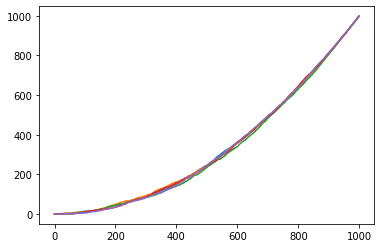
I'm sure that you can say much finer things about the random function you're interested in, but here's a starting point.
Fix $n\in{\mathbb{N}}$ and let $\pi, \sigma$ be permutations selected uniformly at random and independently from $S_{n}$. Define the random function $f_{n}:\{1, 2, ..., n\}\rightarrow{\{0, 1, 2, ..., n\}}$ as follows:
$$
f_{n}(k)=|\{\pi(1), \pi(2), ..., \pi(k)\}\cap{\{\sigma(1), \sigma(2), ..., \sigma(k)\}}|
$$
As Sam Hopkins already pointed out, $f_{n}$ is distributed like $g_{n}$ where $g_{n}:\{1, 2, ..., n\}\rightarrow{\{0, 1, 2, ..., n\}}$ is the function so that $g_{n}(k)$ counts the number of elements of $\{\sigma(1), \sigma(2), ..., \sigma(k)\}$ that are less than or equal to $k$:
$$
g_{n}(k)=|\{1, 2, ..., k\}\cap{\{\sigma(1), \sigma(2), ..., \sigma(k)\}}|
$$
Thus, to understand the behavior of $f_{n}$, it suffices to understand the behavior of $g_{n}$. Now we just do some computations:
$$
\mathbb{E}(g_{n}(k))=\frac{1}{\binom{n}{k}}\sum_{j=1}^{k}j\binom{k}{j}\binom{n-k}{k-j}=\frac{k}{\binom{n}{k}}\sum_{j=1}^{k}j\binom{k-1}{j-1}\binom{n-k}{k-j}=\frac{k\binom{n-1}{k-1}}{\binom{n}{k}}=\frac{k^{2}}{n}
$$
In the first equality, $j$ is the number of elements less than or equal to $k$ found among $\{\sigma(1), \sigma(2), ..., \sigma(n)\}$. The second equality is just algebra. Similarly,
\begin{align*}
\mathbb{E}(g_{n}(k))^{2}&=\frac{1}{\binom{n}{k}}\sum_{j=1}^{k}j^{2}\binom{k}{j}\binom{n-k}{k-j}=\frac{k}{\binom{n}{k}}\sum_{j=1}^{k}j\binom{k-1}{j-1}\binom{n-k}{k-j}= \\ \\
&=\frac{k^{2}}{n}+\frac{k}{\binom{n}{k}}\sum_{j=1}^{k}(j-1)\binom{k-1}{j-1}\binom{n-k}{k-j}=\frac{k^{2}}{n}+\frac{k(k-1)\binom{n-2}{k-2}}{\binom{n}{k}}= \\ \\
&=\frac{k^{2}}{n}+\frac{k^{2}(k-1)^{2}}{n(n-1)}
\end{align*}
Your computer simulations suggested that $g_{n}$ looks deterministic for large $n$. Intuitively, this means it should be concentrated around its mean. We will now make this intuition precise.
Fix $x\in{[0,1]}$. By Chebyshev's inequality, for any fixed $\lambda>0$
$$
\mathbb{P}\Big(\left|\frac{g_{n}(\lfloor{nx}\rfloor)}{n}-\frac{\lfloor{nx}\rfloor^{2}}{n^{2}}\right|>\lambda\Big)\leq{\frac{\mathbb{E}\left(g_{n}(\lfloor{nx}\rfloor)-\frac{\lfloor{nx}\rfloor^{2}}{n}\right)^{2}}{n^{2}\lambda^{2}}}=\lambda^{-2}O(n^{-1})
$$
I've omitted the details, but the last equality just follows by plugging in our formulas for the first and second moment of $g_{n}(k)$ with $k=\lfloor{nx}\rfloor$. Thus, we see that for any fixed $x\in{[0,1]}$,
$$
\frac{g_{n}(\lfloor{nx}\rfloor)}{n}\xrightarrow{(p)}x^{2}
$$
In other words, rescaling the domain and range appropriately, the functions $n^{-1}g_{n}(nx)$ on $[0,1]$ look like $x^{2}$ for large $n$.
Bonus: observe that for any appropriate $n$ and $k$,
$$
g_{n}(k+1)-g_{n}(k)= 0, \hspace{2pt} 1 \hspace{2pt} \text{or} \hspace{4pt} 2
$$
Thus, if we define the rescaled function $n^{-1}g_{n}(nx)$ on $[0,1]$ in any sensible way so that it's continuous- i.e. it is already well- defined at rationals of the form $k/n$. From there, we just linearly interpolate to define it at all values in between- from this observation, it follows that the resulting function will be 2- Lipschitz on $[0,1]$. Additionally, it is clearly bounded above by $1$ and bounded below by $0$. By Arzela- Ascoli, it follows that the measures on $C[0,1]$ induced by the random functions $\big(n^{-1}g_{n}(nx)\big)_{n=1}^{\infty}$ are all supported on the same compact subset of $C[0,1]$. Thus, our collection of random functions, $\big(n^{-1}g_{n}(nx)\big)_{n=1}^{\infty}$, is precompact with respect to the topology of convergence in distribution on $C[0,1]$. Furthermore, by our result from earlier, the marginals of any subsequential limit of this family of random functions is constant. Thus, it follows that:
$$
n^{-1}g_{n}(nx)\xrightarrow{(d)}x^{2} \hspace{5pt}\text{as functions on $C[0,1]$}
$$

