$\newcommand{\vpi}{\varphi}\newcommand\Z{\mathbb Z}$For real $t\ge0$, let $X_t:=mt+W_t$, where $m$ is a real number and $W_\cdot$ is a standard Brownian motion. So, $X_\cdot$ is a drifted Brownian motion starting at $0$ with the constant drift coefficient $m$.
For real $c$, let $T_c:=\min\{t\ge0\colon X_t=c\}$. The probability in question is
\begin{equation*}
P_{t,a,b,m}:=P(T_a\le t,T_b\le t)=1+P(T_a>t,T_b>t)-P(T_a>t)-P(T_b>t),
\end{equation*}
where $-\infty<a<0<b<\infty$ and $t>0$.
By rescaling, without loss of generality $t=1$, because $P_{t,a,b,m}=P_{1,\,a/\sqrt t,\,b\sqrt t,\,m\sqrt t}$. So, it is enough to find
\begin{equation*}
P_{a,b,m}:=P_{1,a,b,m}=1+Q_{a,b}-Q_{a,\infty-}-Q_{-\infty+,b}, \tag{1}
\end{equation*}
where
\begin{equation*}
\begin{aligned}
&Q_{a,b} \\
&:=P(T_a>1,T_b>1) \\
&=P(a<X_s<b\ \forall s\in[0,1]) \\
&=P(a-ms<W_s<b-ms\ \forall s\in[0,1]) \\
&=\int\limits_{a-m}^{b-m}P(a-ms<W_s<b-ms\ \forall s\in[0,1],W_1\in[x,x+dx])) \\
&=\int\limits_{a-m}^{b-m}P(a-(m+x)s<W_s-sW_1<b-(m+x)s\ \forall s\in[0,1], \\
&\, \qquad\qquad\qquad\qquad\qquad\qquad\qquad\qquad\qquad\qquad W_1\in[x,x+dx])) \\
&=\int\limits_{a-m}^{b-m}P(a-(m+x)s<W_s-sW_1<b-(m+x)s\ \forall s\in[0,1]) \\
&\, \qquad\qquad\qquad\qquad\qquad\qquad\qquad\qquad\qquad\qquad P(W_1\in[x,x+dx]) \\
&=\int\limits_{a-m}^{b-m}P(a-(m+x)s<W_s-sW_1<b-(m+x)s\ \forall s\in[0,1], \\
&\, \qquad\qquad\qquad\qquad\qquad\qquad\qquad\qquad\qquad W_1\in[m+x,m+x+dx]) \\
&\, \qquad\qquad\qquad\qquad\qquad\qquad\qquad\qquad\qquad\qquad\times\frac{P(W_1\in[x,x+dx])}{P(W_1\in[m+x,m+x+dx])} \\
&=\int\limits_{a-m}^{b-m}P(a<W_s<b\ \forall s\in[0,1], \ W_1\in[m+x,m+x+dx])
\,\frac{\vpi(x)}{\vpi(m+x)},
\end{aligned}
\end{equation*}
where $\vpi$ is the standard normal pdf; the third and second equalities from the end of the above multiline display follow by the independence of the Brownian bridge $(W_s-sW_1)_{s\in[0,1]}$ from $W_1$.
By multiple reflection (Lévy's triple law -- see e.g. Proposition 6.10.6 or Theorem 6.18),
\begin{equation*}
P(a<W_s<b\ \forall s\in[0,1], \ W_1\in[m+x,m+x+dx])=q_{a,b}(m+x)\,dx,
\end{equation*}
where
\begin{equation*}
q_{a,b}(z):=\sum_{k\in\Z}[\vpi(z+2kh)-\vpi(2b-z+2kh)],
\end{equation*}
\begin{equation*}
h:=b-a,
\end{equation*}
and $z\in(a,b)$.
Taking now the the latter integral in the above multiline display, we get
\begin{equation*}
\begin{aligned}
Q_{a,b}&=Q_{a,b;m}:=\sum_{k\in\Z}e^{-2 h k m} (\Phi (a+2 h k+h-m)-\Phi (a+2 h k-m)) \\
& -\sum_{k\in\Z} e^{2 m (a+h k+h)} (\Phi (a+2 h (k+1)+m)-\Phi (a+2 h k+h+m)),
\end{aligned}
\tag{2}
\end{equation*}
where $\Phi$ is the standard normal cdf.
Now one can find the limits $P(T_a>1)=Q_{a,\infty-}$ and $P(T_b>1)=Q_{-\infty+,b}$ of $Q_{a,b}$ as $b\to\infty$ and as $a\to-\infty$, respectively. Alternatively, these limits can be found directly -- similarly to (but more simply than) $Q_{a,b}$.
Anyway, we get
\begin{equation*}
Q_{-\infty+,b}=P(T_b>1)= \Phi (b-m)-e^{2 m b }\Phi (-b -m)
\end{equation*}
and
\begin{equation*}
Q_{a,\infty-}=P(T_a>1)= \Phi (-a+m)-e^{2 m a }\Phi (a+m);
\end{equation*}
cf. e.g. formula (10.13), p. 13.
Thus, by (1),
\begin{equation*}
\begin{aligned}
P_{a,b;m}&=1+\sum_{k\in\Z}e^{-2 h k m} (\Phi (a+2 h k+h-m)-\Phi (a+2 h k-m)) \\
& -\sum_{k\in\Z} e^{2 m (a+h k+h)} (\Phi (a+2 h (k+1)+m)-\Phi (a+2 h k+h+m)) \\
&- \Phi (b -m)+e^{2 m b }\Phi (-b -m) \\
&-\Phi (-a +m)+e^{2 m a }\Phi (a +m).
\end{aligned}
\end{equation*}
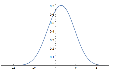
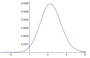
Here is the graph $\{(m,Q_{a,b;m})\colon |m|<5\}$ (above) and $\{(m,P_{a,b;m})\colon-3 < m < 6\}$ (below) for $a=-1$ and $b=2$:


We see that here a small enough positive drift, toward the boundary $b=2$ (which is farther away from the starting point $0$ than the boundary $a=-1$) helps the Brownian motion stay within the two boundaries till time $t=1$. Of course, this should be expected.
The two series in (2) converge very fast: for $a=-1$ and $b=2$, the maximum absolute error seems to be $<2\times10^{-12}$ if the two summations $\sum_{k\in\Z}$ there are each replaced by $\sum_{k=-1}^1$.


