What is the best way to draw curvature?

Question

This is more of a pedagogical question rather than a strictly mathematical one, but I would like to find good ways to visually depict the notion of curvature. It would be preferable to have pictures which have a reasonably simple mathematical formalization and even better if there is a related diagram that explains torsion.

One common picture

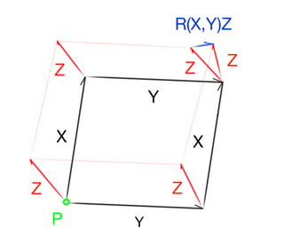
I've often used the above schematic to think about the Riemann curvature tensor $$R(X,Y)Z = \nabla_X \nabla_Y Z - \nabla_Y \nabla_X Z + \nabla_{[X,Y]} Z.$$

This diagram intuitively shows that the curvature involves the difference of covariant derivatives. However, it doesn't really explain why there is another term in the formula (i.e., $\nabla_{[X,Y]} Z$). Also, it takes some work to translate the picture into a precise and correct mathematical formula.

One way to formalize this (suggested by Robert Bryant) is to consider a parallelogram with sides $\epsilon X$ and $\epsilon Y$ in $T_p M$. Then the diagram depicts the parallel transport of $Z$ along the exponential of the sides of the parallelogram. To understand the picture, you parallel transport the vector labelled $R(X,Y)Z$ back to $p$, divide by $\epsilon^2$ and let $\epsilon$ go to $0$. This interpretation is conceptually simple, but has the disadvantage that the top and right hand sides of the parallelogram are not geodesics, so we cannot use this interpretation to draw a similar diagram for torsion.

There are other ways to formalize this diagram, and it would be interesting to hear other simple and correct explanations for this picture (or any variation of it).

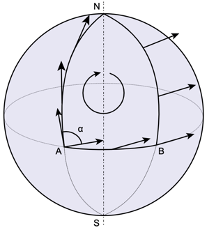
Another common picture

Another commonly used picture to explain curvature is a spherical triangle with two vertices on the equator and a third at a pole. This intuitively shows that curvature gives rise to holonomy, but also relies on the global geometry of the sphere. In other words, it doesn't really depict curvature as "local holonomy."

Answer 1

The best way I know to illustrate the notion of curvature is via Toponogov's theorem. We can compare any (geodesic) triangle in a Riemannian manifold $M$ with one with the same edge lengths in Euclidean plane $R^2$. The (sectional) curvature of $M$ is positive (resp. negative) provided that all its triangles are fatter (resp. thinner) than the comparison triangle. More precisely, this means that the distance between each vertex and the midpoint of the opposite side is bigger (resp. smaller) than the corresponding distance in the comparison triangle.

Answer 2

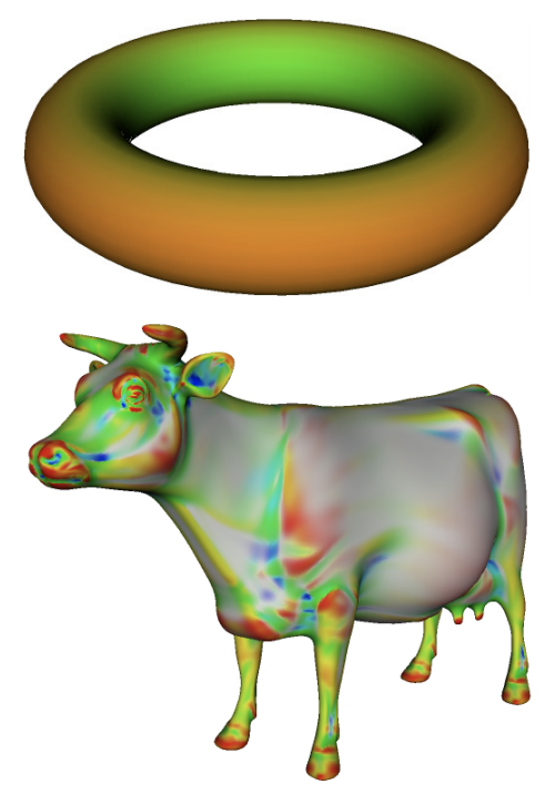
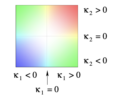
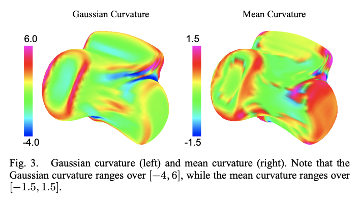
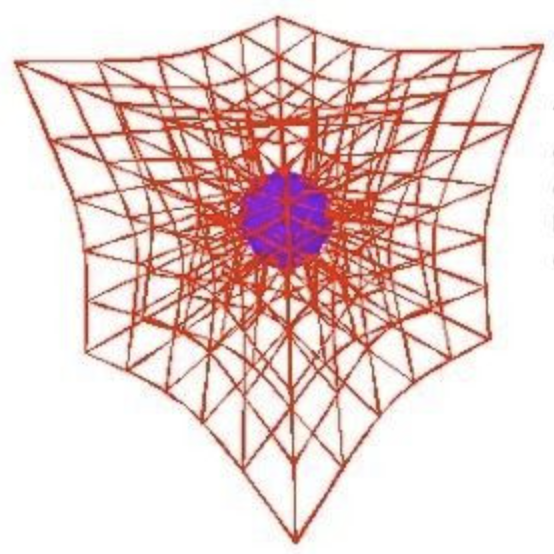
With advances in discrete differential geometry, it is now nearly routine to compute curvature on meshed surfaces. Here are two of many possible color-coded examples.

---

     

---

Rusinkiewicz, Szymon. "Estimating curvatures and their derivatives on triangle meshes." In Proceedings. 2nd International Symposium on 3D Data Processing, Visualization and Transmission, 2004. 3DPVT 2004., pp. 486-493. IEEE, 2004. Fig. 4 (detail). DOI.

---

     

---

Gatzke, Timothy, Cindy Grimm, Michael Garland, and Steve Zelinka. "Curvature maps for local shape comparison." In International Conference on Shape Modeling and Applications 2005 (SMI'05), pp. 244-253. IEEE, 2005. DOI.

(Added in response to comment:)

Found at this link (originator unknown.)

Answer 3

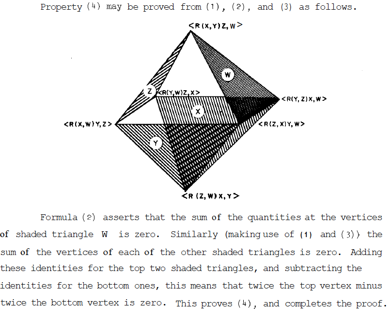
This is not what you're looking for, but I always remember Milnor's diagram in Chapter 9 of his book on Morse Theory describing the symmetries of the curvature tensor.

Answer 4

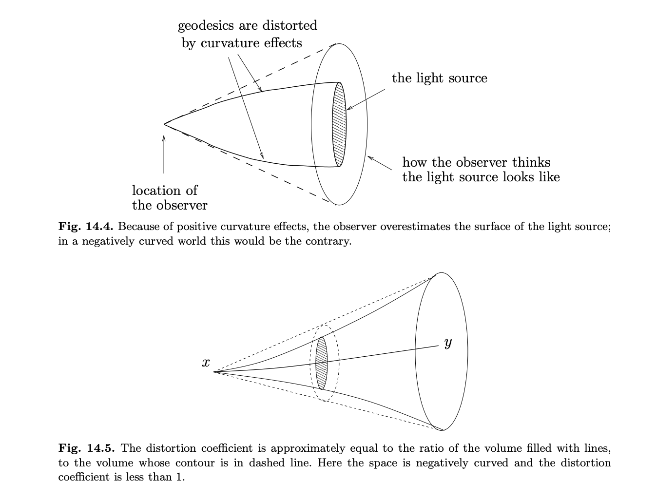
Mohammed Ghomi's answer reminds me of a related picture that Cedric Villani drew to depict Ricci curvature ([1] Chapter 14). Similar to the $\operatorname{CAT}(\kappa)$ inequality, this idea can be used to derive notions of Ricci curvature for more general metric measure spaces.

[1] Villani, Cédric, Optimal transport. Old and new, Grundlehren der Mathematischen Wissenschaften 338. Berlin: Springer (ISBN 978-3-540-71049-3/hbk). xxii, 973 p. (2009). ZBL1156.53003.

Answer 5

This is a very similar picture to that in the answer by Gabe, but concerning the sectional curvature of a Riemannian metric. Consider a point $p\in M$, and a plane $V\subset T_pM.$ For small radius $r$ consider the image under the exponential map of the circle of radius $r$ in $V$ centered at $0$. This is a closed curve $C(r)$ in the manifold and its length behaves like $$L(C(r))\sim 2\pi r (1-\frac{1}{6}Kr^2\dots)$$ for $r$ small. It turns out that $K$ is the sectional curvature of the plane $V\subset T_pM.$ Of course, pictures for 2-dimensional Riemannian manifolds in 3-dimensional space are particularly useful to see what curvature does. To prove this expansion of the length just use the Taylor expansion of the metric in normal coordinates. If I am not mistaken, this was used by Riemann to define curvature (of a Riemannian manifold).

Answer 6

Curvature can be very easily pictured using ‘geodesic quadrilateral gaps’, which can be more generally used to recover the torsion tensor, and if the torsion is identically zero, then the curvature tensor, for a manifold equipped with an affine connection.

In the special case of an oriented Riemannian surface $(M,g)$ with its Riemannian connection $\nabla$, this works as follows to pictorially give us the Gaussian curvature $\kappa(P_0)$ at any point $P_0 \in M$. Travel along a geodesic from $P_0$ in the starting direction given by a unit vector $u\in T_{P_0}M$, and take the point $P_1$ on it at a small distance $s$ from $P_0$. Turn left in $90$ degrees, and follow the geodesic in that direction for the same distance $s$ to arrive at a point $P_2$. Iterate the left turn and the travel along the geodesic for distance $s$ twice more, to successively arrive at points $P_3$ and $P_4$. If the surface was flat, and $s$ small enough, then we would have traveled along a closed geodesic quadrilateral and arrived back at the starting point, that is, $P_4 = P_0$. But if the curvature is non zero, then the vector $P_4 - P_0$ (which you can define in terms of a local smooth embedding of $M$ in a higher dimensional vector space) is non-zero, and satisfies the following formula. Let $v\in T_{P_0}M$ be the vector such that $(u,v)$ is a right-handed orthonormal basis for $T_{P_0}M$. Then $$\lim_{s\to 0}\, {P_4 - P_0 \over s^3} = {\kappa(P_0) \over 2}(u - v).$$

More generally, let there be give a pair $(M,\nabla)$ where $M$ is a smooth manifold and $\nabla$ is a connection on $TM$. Consider any $P\in M$ and a pair of vectors $u,v \in T_PM$. From the triple $(P,u,v)$ and a small real number $s$, we can make a new triple $(P',u',v')$ as follows. Take the geodesic from $P$ with starting tangent vector $u$, and let $P'$ be the point on it where the affine parameter takes the value $s$ (where the parameter has value $0$ at $P$). Let $u',v' \in T_{P'}M$ where $u'$ is parallel transport of $v$ and $v'$ is $(-1)$-times the parallel transport of $u$ along this geodesic. Starting with a triple $(P,u,v)$ for which $P = P_0$, and iterating the above, we get an open geodesic quadrilateral with vertices $P_0$, $P_1 = (P_0)'$, $P_2 = (P_1)'$, $P_3 = (P_2)'$ and $P_4= (P_3)'$. The quadrilateral is closed if $P_4 = P_0$. But in general, we have the formula

$$\lim_{s\to 0}\,{P_4 - P_0\over s^2} = - T(u,v)$$

where $T(u,v) = \nabla_uv - \nabla_vu - [u,v]$ is the torsion tensor. If the torsion tensor $T$ is identically zero on $M$, then the gap $P_4 - P_0$ is given in terms of the Riemann curvature tensor by the formula

$$\lim_{s\to 0}\,{P_4 - P_0\over s^3} = {1\over 2}R(u,v)(u+v)$$

where by definition $R(u,v)(w) = \nabla_u\nabla_vw - \nabla_v\nabla_uw - \nabla_{[u,v]}w$. The above formula can be ‘inverted’ to recover the curvature tensor when the torsion is identically zero, as the tensor $R(u,v)(w)$ can be recovered uniquely from the tensor $R(u,v)(u+v)$ using the symmetries of $R(u,v)(w)$.

The above results are proved in arXiv:1910.06615, which is written in an expository style.

Answer 7

Personally, I think the best way to illustrate curvature is to start from the simplest case. This is how Hilbert illustrated it in his book, Geometry and the Imagination.

1. The simplest curve is the the straight line and its curvature obviously should be zero.

2. The next simplest curve is the circle. Since the only invariant of a circle is the radius, the curvature must involve this. The larger the circle, the less curved it is. The simplest way to describe this is to say that curvature is the reciprocal of the radius.

3. For any other curve we measure its curvature by fitting a circle to it and calling its radius, the radius of curvature.

Of course this leaves unexplained how to actually find this fitting circle. Both Newton and Liebniz provided different but equivalent method: Basically, take two points on either side of the chosen point and draw the tangent there. Then draw the normals. Where they intersect is the approximate centre of this circle. Then by taking the limits of both points approaching the chosen point we find the true centre and hence radius of curvature.

I like this because it directly connects our intuitive notion of curvature to its formalisation. Hilbert doesn't describe how to generalise this to higher dimensions, but presumably it's a question of fitting ellipsoids...

For example, on a surface, we would get a fitting ellipse whose major and semi-major axes will be the principal axes of curvature. Gauss then showed that the product of these the two radii, the Gaussian curvature, was independent of the embedding of the surface in Euclidean space - his theorem egregium, his 'remarkable theorem'. This inaugurated the era of intrinsic geometry as opposed to extrinsic geometry where we consider a geometrical object embedded in another.

It's probably worthwhile to add that this product is - upto a constant of proportionality - the area of the bounding rectangle. And this hints at the usefulness of tensors in dealing with curvature as tensors geometrically represent volumes (that is, upto rotations and shears).

Of course it is a mistake to think intrinsic geometry is the final word on geometry. After all, the theory of bundles (and of cobundles), as used in gauge theory and homology/cohomology shows that it is equally important to keep the extrinsic view in mind.

More practically, we can see this with the Möbius strip. Intrinsically, it can only have two twists; the trivial one and the half-twist; extrinsically, there is a natural numbers worth of full twists and of half twists. This is important in the theory of spin in physics.