1
$\begingroup$

Update: Oops! This is a stupid question and should be closed. The definition of the probability space that contains events $A_i$ requires using a single random stream.

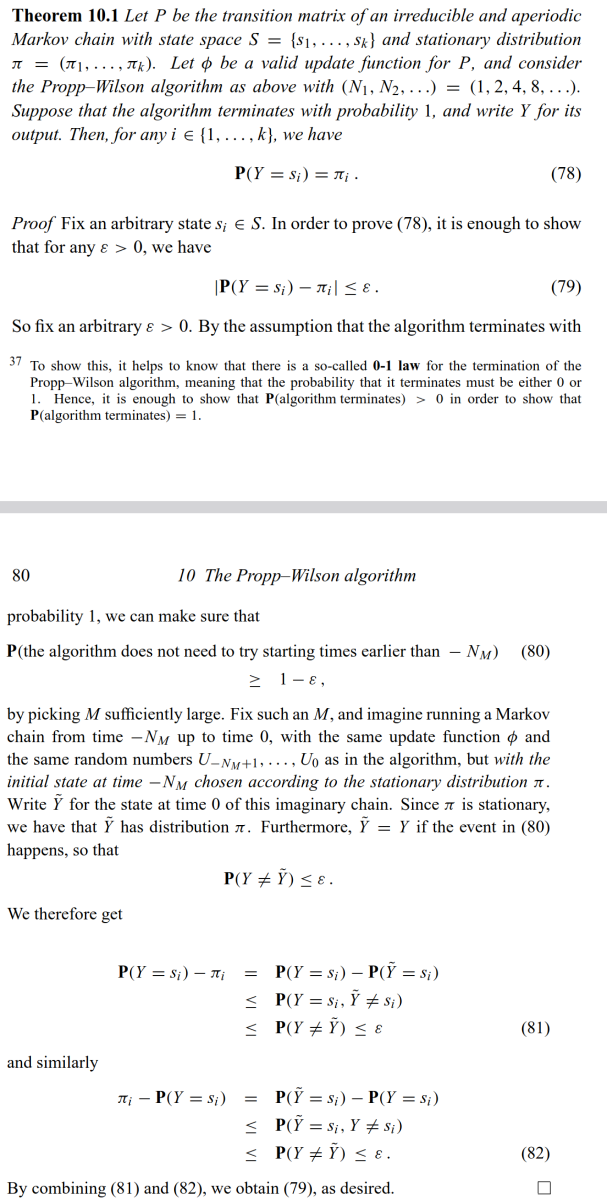
I have difficulties understanding the proof of the Propp-Wilson algorithm in the book "Finite Markov Chains and Algorithmic Applications" 1 by Olle Häggström. I'm not sure how the "reusing old randomness" is used in the proof given in the book.

The proof is on page 79, below the theorem 10.1. It goes as follows:

enter image description here

My question is: Where is the use of "reusing old randomness" in the proof? I intuitively understand that if one generates completely new random numbers in each round, the algorithm will be more likely to over-sample those paths that couple together quickly. Hence the sampling is biased. However, I can't see how this is used in the proof.

1. http://cms.dm.uba.ar/academico/materias/verano2016/probabilidades_y_estadistica_C/Haggstrom-Finite%20Markov%20chains%20and%20algorithm%20applications.pdf

$\endgroup$
1
  • $\begingroup$ How would you couple from the future the chains in $\{1,2,3\}$ if the transitions are given by $P(1\to2)=1$, $P(2\to 3)=1/2=P(2\to 1)$, $P(3\to1)=1$? Can the chains meet first at $2$ if they are coupled forward? Work out your proof that coupling from the future succeeds on this example to figure out where the proof cannot hold. $\endgroup$
    – jlewk
    Commented Dec 1, 2023 at 4:31

1 Answer 1

4
$\begingroup$

The claim that $P(Y=\tilde Y)=1$ is incorrect. But I do not see this claim in the book you linked to.

Yes, the algorithm will oversample some states if one does not "reuse previous randomness". With the transition matrix on state space $\{0,1,2\}$ given by $$\begin{pmatrix} .5 & .5 & 0 \\ .5 & 0 & .5 \\ 0 & .5 & .5 \end{pmatrix} $$ and moving the chain according to the random function $f$ defined by \begin{align} P(f(0)&=1, f(1)=2, f(2)=2) = 1/2, \\P(f(0)&=0, f(1)=0, f(2)=1) = 1/2, \end{align} the algorithm that "throws away" previous randomness does oversample the two extreme states $\{0,2\}$. This can be seen by computing the probability that the algorithm ouputs $\{0,2\}$ at times $t\in\{1,2\}$, which is already too big compared to $\pi(0)+\pi(2)$.

$\endgroup$
3
  • $\begingroup$ Thank you. I know the counterexamples that demonstrate why one should reuse randomness, and why coupling into the future will not work. What puzzled me is how they are used in the proof, because the proof itself did not explicitly say "Since we are using the old randomness, we have blahblah..." $\endgroup$
    – zemora
    Commented Dec 1, 2023 at 6:57
  • 1
    $\begingroup$ If all previous randomness is thrown away everytime $i$ is increased, how to pick the randomness to define $\tilde Y$? We have now several candidates since the randomness indexed at $-1$ has been resampled $i$ times. By not throwing away, $\tilde Y$ is well defined. $\endgroup$
    – jlewk
    Commented Dec 1, 2023 at 7:43
  • $\begingroup$ Hi, I have edited my question. I guess the ambiguity of $\tilde{Y}$ is not the main problem, because one can define $\tilde{Y}$ by using the last random stream that succeeded in producing a coupling? Isn't the use of old randomness lies in the argument "by the arbitrariness of $\epsilon$"? Because resuing old randomness ensures that once we go further into the past, all chains will still couple at $Y$, hence the left hand of $|P(Y=s_i)-\pi(s_i)|\leq\epsilon$ does not change? $\endgroup$
    – zemora
    Commented Dec 16, 2023 at 3:30

You must log in to answer this question.

Not the answer you're looking for? Browse other questions tagged .