added 171 characters in body
Source Link
zemora
  • 565
  • 2
  • 11

Update: Oops! This is a stupid question and should be closed. The definition of the probability space that contains events $A_i$ requires using a single random stream.

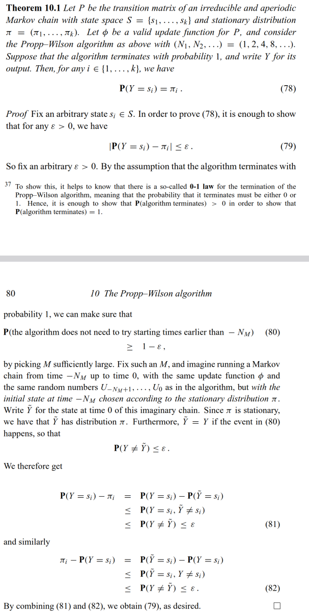
I have difficulties understanding the proof of the Propp-Wilson algorithm in the book "Finite Markov Chains and Algorithmic Applications" 1 by Olle Häggström. I'm not sure how the "reusing old randomness" is used in the proof given in the book.

The proof is on page 79, below the theorem 10.1. It goes as follows:

enter image description here

My question is: Where is the use of "reusing old randomness" in the proof? I intuitively understand that if one generates completely new random numbers in each round, the algorithm will be more likely to over-sample those paths that couple together quickly. Hence the sampling is biased. However, I can't see how this is used in the proof.

1. http://cms.dm.uba.ar/academico/materias/verano2016/probabilidades_y_estadistica_C/Haggstrom-Finite%20Markov%20chains%20and%20algorithm%20applications.pdf

Update: Oops! This is a stupid question and should be closed. The definition of the probability space that contains events $A_i$ requires using a single random stream.

I have difficulties understanding the proof of the Propp-Wilson algorithm in the book "Finite Markov Chains and Algorithmic Applications" 1 by Olle Häggström. I'm not sure how the "reusing old randomness" is used in the proof given in the book.

The proof is on page 79, below the theorem 10.1. It goes as follows:

enter image description here

My question is: Where is the use of "reusing old randomness" in the proof? I intuitively understand that if one generates completely new random numbers in each round, the algorithm will be more likely to over-sample those paths that couple together quickly. Hence the sampling is biased. However, I can't see how this is used in the proof.

1. http://cms.dm.uba.ar/academico/materias/verano2016/probabilidades_y_estadistica_C/Haggstrom-Finite%20Markov%20chains%20and%20algorithm%20applications.pdf

deleted 2048 characters in body
Source Link
zemora
  • 565
  • 2
  • 11

I have difficulties understanding the proof of the Propp-Wilson algorithm in the book "Finite Markov Chains and Algorithmic Applications" [1]1 by Olle Häggström. I'm not sure how the two key gradients "coupling from the past" and "reusing old randomness" areis used in the proof given in the book.

The proof is on page 79, below the theorem 10.1. It goes as follows:

  1. Let $$A = \{ \text{the algorithm terminates in finite time}\}$$ be the event that the algorithm finishes in finite time, and $$A_i = \{ \text{the algorithm need not to try starting times earlier than} -N_i\}.$$ where $N_i=2^i$. Then $P(A_i)\uparrow P(A)=1$.
  2. In each round, the algorithm runs all $|S|$ chains from time $-N_i$, using one same random stream $\{U_i, 1\leq i\leq N_i\}$ for all chains, and checks if these chains are coupled together at time 0. If they do, then output the final state; otherwise, increase $i$ by one, restart all chains from time $-N_{i+1}$, generating new random stream for $[-N_{i+1}, -N_i)$, while using the old randomness for $[-N_i, 1]$.
  3. Repeat 2 until all chains are coupled for some $i$.
  4. Suppose the final state returned by the algorithm is $Y$, and let $\tilde{Y}$ be another chain that also starts from time $-N_i$, whose initial distribution is the stationary distribution $\pi$, then $\tilde{Y}$ will also be coupled together with the $|S|$ chains, Olleh Häggström argued that $P(Y=s_i)=\pi(s_i)$ for any state $s_i\in S$, hence $Y$ obeys the stationary distribution $\pi$.

My questions are:enter image description here
  • Where is the use of "reusing old randomness" in the proof? I have an intuitive understanding that if one generates completely new random numbers in each round, then the algorithm will be more likely to over-sample those paths that couple together quickly. Hence the sampling is biased. However, I can't see how this is used in the proof.

  • Why coupling into the future will fail? I tried to modify the proof of Theorem10.1 to make it also work the coupling into the future as follows:

    i) Run all $|S|$ copies of chains starting from time 0 using the same random stream, into the future, and also run an independent copy from time 0, whose initial state is sampled from the stationary distribution.

    ii) Choose $N_m$ large enough so that the probability of all $|S|$ chains couple together between $[0, N_m]$ is larger than $1-\epsilon$.

    iii) Mimic the proof to prove that $P(Y=s_i) = \pi(s_i)$.

It seems to me thereMy question is no obvious error: Where is the use of "reusing old randomness" in the procedure.proof? I suspectintuitively understand that the problem liesif one generates completely new random numbers in the statement that when choosing $N_m$ largereach round, both the random variable $Y$ and $\epsilon$algorithm will be changed in coupling into the future (which does not happen for coupling from the past, in coupling frommore likely to over-sample those paths that couple together quickly. Hence the past, only $\epsilon$sampling is changedbiased. However, while $Y$I can't see how this is not)used in the proof.

[1]1. http://cms.dm.uba.ar/academico/materias/verano2016/probabilidades_y_estadistica_C/Haggstrom-Finite%20Markov%20chains%20and%20algorithm%20applications.pdf

I have difficulties understanding the proof of the Propp-Wilson algorithm in the book "Finite Markov Chains and Algorithmic Applications" [1] by Olle Häggström. I'm not sure how the two key gradients "coupling from the past" and "reusing old randomness" are used in the proof given in the book.

The proof is on page 79, below the theorem 10.1. It goes as follows:

  1. Let $$A = \{ \text{the algorithm terminates in finite time}\}$$ be the event that the algorithm finishes in finite time, and $$A_i = \{ \text{the algorithm need not to try starting times earlier than} -N_i\}.$$ where $N_i=2^i$. Then $P(A_i)\uparrow P(A)=1$.
  2. In each round, the algorithm runs all $|S|$ chains from time $-N_i$, using one same random stream $\{U_i, 1\leq i\leq N_i\}$ for all chains, and checks if these chains are coupled together at time 0. If they do, then output the final state; otherwise, increase $i$ by one, restart all chains from time $-N_{i+1}$, generating new random stream for $[-N_{i+1}, -N_i)$, while using the old randomness for $[-N_i, 1]$.
  3. Repeat 2 until all chains are coupled for some $i$.
  4. Suppose the final state returned by the algorithm is $Y$, and let $\tilde{Y}$ be another chain that also starts from time $-N_i$, whose initial distribution is the stationary distribution $\pi$, then $\tilde{Y}$ will also be coupled together with the $|S|$ chains, Olleh Häggström argued that $P(Y=s_i)=\pi(s_i)$ for any state $s_i\in S$, hence $Y$ obeys the stationary distribution $\pi$.

My questions are:

  • Where is the use of "reusing old randomness" in the proof? I have an intuitive understanding that if one generates completely new random numbers in each round, then the algorithm will be more likely to over-sample those paths that couple together quickly. Hence the sampling is biased. However, I can't see how this is used in the proof.

  • Why coupling into the future will fail? I tried to modify the proof of Theorem10.1 to make it also work the coupling into the future as follows:

    i) Run all $|S|$ copies of chains starting from time 0 using the same random stream, into the future, and also run an independent copy from time 0, whose initial state is sampled from the stationary distribution.

    ii) Choose $N_m$ large enough so that the probability of all $|S|$ chains couple together between $[0, N_m]$ is larger than $1-\epsilon$.

    iii) Mimic the proof to prove that $P(Y=s_i) = \pi(s_i)$.

It seems to me there is no obvious error in the procedure. I suspect that the problem lies in the statement that when choosing $N_m$ larger, both the random variable $Y$ and $\epsilon$ will be changed in coupling into the future (which does not happen for coupling from the past, in coupling from the past, only $\epsilon$ is changed, while $Y$ is not).

[1]. http://cms.dm.uba.ar/academico/materias/verano2016/probabilidades_y_estadistica_C/Haggstrom-Finite%20Markov%20chains%20and%20algorithm%20applications.pdf

I have difficulties understanding the proof of the Propp-Wilson algorithm in the book "Finite Markov Chains and Algorithmic Applications" 1 by Olle Häggström. I'm not sure how the "reusing old randomness" is used in the proof given in the book.

The proof is on page 79, below the theorem 10.1. It goes as follows:

enter image description here

My question is: Where is the use of "reusing old randomness" in the proof? I intuitively understand that if one generates completely new random numbers in each round, the algorithm will be more likely to over-sample those paths that couple together quickly. Hence the sampling is biased. However, I can't see how this is used in the proof.

1. http://cms.dm.uba.ar/academico/materias/verano2016/probabilidades_y_estadistica_C/Haggstrom-Finite%20Markov%20chains%20and%20algorithm%20applications.pdf

added 25 characters in body
Source Link
zemora
  • 565
  • 2
  • 11

I have difficulties in understanding the proof of the Propp-Wilson algorithm in the book "Finite Markov Chains and Algorithmic Applications" [1] by Olle Häggström. I'm not sure how the two key gradients "coupling from the past" and "reusing old randomness" are used in the proof given in the book.

The proof is on page 79, below the theorem 10.1. It goes as follows:

  1. Let $$A = \{ \text{the algorithm terminates in finite time}\}$$ be the event that the algorithm finishes in finite time, and $$A_i = \{ \text{the algorithm need not to try starting times earlier than} -N_i\}.$$ where $N_i=2^i$. Then $P(A_i)\uparrow P(A)=1$.
  2. In each round, the algorithm runs all $|S|$ chains from time $-N_i$, using one same random stream $\{U_i, 1\leq i\leq N_i\}$ for all chains, and checkchecks if these chains are coupled together at time 0. If they do, then output the final state; otherwise, increase $i$ by one, restart all chains from time $-N_{i+1}$, generating new random stream for $[-N_{i+1}, -N_i)$, while using the old randomness for $[-N_i, 1]$.
  3. Repeat 2 until all chains are coupled for some $i$.
  4. Suppose the final state retunedreturned by the algorithm is $Y$, and let $\tilde{Y}$ be another chain that also starts from time $-N_i$, whose initial distribution is the stationary distribution $\pi$, then $\tilde{Y}$ will also be coupled together with the $|S|$ chains, Olleh Häggström argued that $P(Y=\tilde{Y})=1$$P(Y=s_i)=\pi(s_i)$ for any state $s_i\in S$, hence $Y$ obeys the stationary distribution $\pi$.

My questions are:

  • Where is the use of "reusing old randomness" in the proof? I have an intuitive understanding that if one generates completely new random numbers in each round, then the algorithm will be more likely to over-sample those paths that couple together quickly. Hence the sampling is biased. However, I can't see how this is used in the proof.

  • Why coupling into the future will fail? I tried to modify the proof of Theorem10.1 to make it also work the coupling into the future as follows:

    i) Run all $|S|$ copies of chains starting from time 0 using the same random stream, into the future, and also run an independent copy from time 0, whose initial state is sampled from the stationary distribution.

    ii) Choose $N_m$ large enough so that the probability of all $|S|$ chains couple together between $[0, N_m]$ is larger than $1-\epsilon$.

    iii) Mimic the proof to prove that $P(Y=s_i) = \pi(s_i)$.

It seems to me there is no obvious error in the procedure. I suspect that the problem lies in the statement that when choosing $N_m$ larger, both the random variable $Y$ and $\epsilon$ will be changed in coupling into the future (which does not happen for coupling from the past, in coupling from the past, only $\epsilon$ is changed, while $Y$ is not).

[1]. http://cms.dm.uba.ar/academico/materias/verano2016/probabilidades_y_estadistica_C/Haggstrom-Finite%20Markov%20chains%20and%20algorithm%20applications.pdf

I have difficulties in understanding the proof of the Propp-Wilson algorithm in the book "Finite Markov Chains and Algorithmic Applications" [1] by Olle Häggström. I'm not sure how the two key gradients "coupling from the past" and "reusing old randomness" are used in the proof given in the book.

The proof is on page 79, below the theorem 10.1. It goes as follows:

  1. Let $$A = \{ \text{the algorithm terminates in finite time}\}$$ be the event that the algorithm finishes in finite time, and $$A_i = \{ \text{the algorithm need not to try starting times earlier than} -N_i\}.$$ where $N_i=2^i$. Then $P(A_i)\uparrow P(A)=1$.
  2. In each round, the algorithm runs all $|S|$ chains from time $-N_i$, using one same random stream $\{U_i, 1\leq i\leq N_i\}$ for all chains, and check if these chains are coupled together at time 0. If they do, then output the final state; otherwise, increase $i$ by one, restart all chains from time $-N_{i+1}$, generating new random stream for $[-N_{i+1}, -N_i)$, while using the old randomness for $[-N_i, 1]$.
  3. Repeat 2 until all chains are coupled for some $i$.
  4. Suppose the final state retuned by the algorithm is $Y$, and let $\tilde{Y}$ be another chain that also starts from time $-N_i$, whose initial distribution is the stationary distribution $\pi$, then $\tilde{Y}$ will also be coupled together with the $|S|$ chains, Olleh Häggström argued that $P(Y=\tilde{Y})=1$, hence $Y$ obeys the stationary distribution $\pi$.

My questions are:

  • Where is the use of "reusing old randomness" in the proof? I have an intuitive understanding that if one generates completely new random numbers in each round, then the algorithm will be more likely to over-sample those paths that couple together quickly. Hence the sampling is biased. However, I can't see how this is used in the proof.

  • Why coupling into the future will fail? I tried to modify the proof of Theorem10.1 to make it also work the coupling into the future as follows:

    i) Run all $|S|$ copies of chains starting from time 0 using the same random stream, into the future, and also run an independent copy from time 0, whose initial state is sampled from the stationary distribution.

    ii) Choose $N_m$ large enough so that the probability of all $|S|$ chains couple together between $[0, N_m]$ is larger than $1-\epsilon$.

    iii) Mimic the proof to prove that $P(Y=s_i) = \pi(s_i)$.

It seems to me there is no obvious error in the procedure. I suspect that the problem lies in the statement that when choosing $N_m$ larger, both the random variable $Y$ and $\epsilon$ will be changed in coupling into the future (which does not happen for coupling from the past, in coupling from the past, only $\epsilon$ is changed, while $Y$ is not).

[1]. http://cms.dm.uba.ar/academico/materias/verano2016/probabilidades_y_estadistica_C/Haggstrom-Finite%20Markov%20chains%20and%20algorithm%20applications.pdf

I have difficulties understanding the proof of the Propp-Wilson algorithm in the book "Finite Markov Chains and Algorithmic Applications" [1] by Olle Häggström. I'm not sure how the two key gradients "coupling from the past" and "reusing old randomness" are used in the proof given in the book.

The proof is on page 79, below the theorem 10.1. It goes as follows:

  1. Let $$A = \{ \text{the algorithm terminates in finite time}\}$$ be the event that the algorithm finishes in finite time, and $$A_i = \{ \text{the algorithm need not to try starting times earlier than} -N_i\}.$$ where $N_i=2^i$. Then $P(A_i)\uparrow P(A)=1$.
  2. In each round, the algorithm runs all $|S|$ chains from time $-N_i$, using one same random stream $\{U_i, 1\leq i\leq N_i\}$ for all chains, and checks if these chains are coupled together at time 0. If they do, then output the final state; otherwise, increase $i$ by one, restart all chains from time $-N_{i+1}$, generating new random stream for $[-N_{i+1}, -N_i)$, while using the old randomness for $[-N_i, 1]$.
  3. Repeat 2 until all chains are coupled for some $i$.
  4. Suppose the final state returned by the algorithm is $Y$, and let $\tilde{Y}$ be another chain that also starts from time $-N_i$, whose initial distribution is the stationary distribution $\pi$, then $\tilde{Y}$ will also be coupled together with the $|S|$ chains, Olleh Häggström argued that $P(Y=s_i)=\pi(s_i)$ for any state $s_i\in S$, hence $Y$ obeys the stationary distribution $\pi$.

My questions are:

  • Where is the use of "reusing old randomness" in the proof? I have an intuitive understanding that if one generates completely new random numbers in each round, then the algorithm will be more likely to over-sample those paths that couple together quickly. Hence the sampling is biased. However, I can't see how this is used in the proof.

  • Why coupling into the future will fail? I tried to modify the proof of Theorem10.1 to make it also work the coupling into the future as follows:

    i) Run all $|S|$ copies of chains starting from time 0 using the same random stream, into the future, and also run an independent copy from time 0, whose initial state is sampled from the stationary distribution.

    ii) Choose $N_m$ large enough so that the probability of all $|S|$ chains couple together between $[0, N_m]$ is larger than $1-\epsilon$.

    iii) Mimic the proof to prove that $P(Y=s_i) = \pi(s_i)$.

It seems to me there is no obvious error in the procedure. I suspect that the problem lies in the statement that when choosing $N_m$ larger, both the random variable $Y$ and $\epsilon$ will be changed in coupling into the future (which does not happen for coupling from the past, in coupling from the past, only $\epsilon$ is changed, while $Y$ is not).

[1]. http://cms.dm.uba.ar/academico/materias/verano2016/probabilidades_y_estadistica_C/Haggstrom-Finite%20Markov%20chains%20and%20algorithm%20applications.pdf

Source Link
zemora
  • 565
  • 2
  • 11
Loading