On a von Bahr–Esseen-type inequality for pairwise independent zero-mean random variables

Question

For $p\in(1,2)$, let $C_p$ be the smallest constant factor $C$ in the von Bahr–Esseen-type inequality \begin{equation}\label{eq:pair}\tag{1} E\Bigl\lvert\sum_{j=1}^n X_j\Bigr\rvert^p\le C\sum_{j=1}^n E\lvert X_j\rvert^p \end{equation} for all natural $n$ and all pairwise independent zero-mean real-valued random variables $X_1,\dotsc,X_n$.

According to Theorem 4.4, \begin{equation}\label{eq:C<} C_p\le\frac4{2-p}. \end{equation}

---

Questions:

Q1: Is it true that $\sup_{p\in(1,2)}C_p<\infty$?

Q2: Is it true that $\inf_{p\in(1,2)}\big((2-p)C_p\big)>0$?

Q3: Is there a simply described asymptotic behavior of $C_p$ as $p\uparrow2$?

Q3a: Is there a simply described asymptotic behavior of the smallest constant factor $C$ in \eqref{eq:pair} as $p\uparrow2$ assuming also that each $X_j$ is symmetrically distributed?

Any correct and complete answer to any one of these four questions will be considered a correct and complete answer to this entire post.

Of course, an answer to Q3 or Q3a will also be an answer to Q1 and Q2. Also, a positive answer to Q1 would imply a negative answer to Q2, and a positive answer to Q2 would imply a negative answer to Q1.

By Proposition 1.8 (iii), letting $D_p$ denote the smallest constant factor $C$ in \eqref{eq:pair} for all natural $n$ and all completely independent zero-mean real-valued random variables $X_1,\dotsc,X_n$, we have $D_p\to1$ as $p\uparrow2$. More generally, here we may assume that the $X_j$'s are martingale-differences (or, even, satisfy another, slightly more general condition).

Answer 1

Here is a positive answer to Q1.

Step 1: Without loss of generality, each $X_i$ is symmetrically distributed. Indeed, consider an independent copy $X_i'$ of the family $X_i$ with the same joint distribution. Then $$ E\left|\sum_i X_i\right|^p\le E\left|\sum_i (X_i-X_i')\right|^p $$ (only the mean $0$ property and the convexity of $x\mapsto |x|^p$ are used here) while $$ E|X_i-X_i'|^p\le 2^p E|X_i|^p $$ and $X_i-X_i'$ are still pairwise independent.

Now choose $Q>0$ so that $Q^{2-p}=2$. Clearly, $Q\ge 2$. Define $X_{i,k}=X_i$ if $Q^k\le|X_i|< Q^{k+1}$ and $0$ otherwise ($k\in\mathbb Z$). Also denote by $Y_{\ell,k}$ the characteristic function of the event $Q^{\ell+k}\le\left|\sum_i X_{i,k}\right|<Q^{\ell+k+1}$ ($\ell\in\mathbb Z$).

Step 2: The key estimates: When $\ell\ge 0$, we have $$ E\left[Y_{\ell,k}\left|\sum_i X_{i,k}\right|^p\right]\le Q^{(p-2)(\ell+k)}E\left|\sum_i X_{i,k}\right|^2 \\ =Q^{(p-2)(\ell+k)}\sum_i E\left|X_{i,k}\right|^2\le 2Q^{(p-2)\ell}\sum_i E|X_{i,k}|^p=2^{1-\ell}\sum_i E|X_{i,k}|^p $$ because $Q^{(p-2)k}|x|^2\le 2|x|^p$ when $x=0$ or $Q^k\le|x|<Q^{k+1}$.

If $\ell<0$, then $$ E\left[Y_{\ell,k}\left|\sum_i X_{i,k}\right|^p\right]\le Q^{p(\ell+1)}\sum_i E|X_{i,k}|^p\le 2^{1+\ell}\sum_i E|X_{i,k}|^p $$ merely because the absolute value of the sum (if not zero) is less than $Q^{\ell+1}$ times the absolute value of any non-zero term in it.

Step 3: Summing over k with fixed $\ell$. The crucial point here is that if we have any sequence of random variables $F_k$ such that the absolute value of $F_k$ is either $0$ or between $Q^{\ell+k}$ and $Q^{\ell+k+1}$, then $$ \left|\sum_k F_k\right|^p\le 4^p\max_k|F_k|^p\le 4^p\sum_k|F_k|^p\,. $$
It follows that $$ E\left|\sum_k \left[Y_{\ell,k}\sum_i X_{i,k}\right]\right|^p\le 4^p\cdot 2^{1-|\ell|}\sum_k \sum_i E|X_{i,k}|^p= 4^p\cdot 2^{1-|\ell|}\sum_i E|X_{i}|^p\,, $$ i.e., $$ \left\|\sum_k \left[Y_{\ell,k}\sum_i X_{i,k}\right]\right\|_{L^p}\le 4\cdot 2^{(1-|\ell|)/p}\left[\sum_i E|X_{i}|^p\right]^{1/p}\,. $$

Step 4: Use Minkowski's inequality when summing over $\ell$ now and observe that $$ \sum_\ell\sum_k \left[Y_{\ell,k}\sum_i X_{i,k}\right]=\sum_i X_i\,. $$

Edit: Chasing the constant.

The technique outlined above is often useful as a replacement of interpolation when the latter fails to work directly for some reason. However, in this case we can utilize the complex interpolation tool in its original form for symmetric random variables. Here is how it can be done (I'll even assume that $X_i$ are complex, though it does not matter):

Normalize the variables so that $\sum_i E|X_i|^p=1$. Write each $X_i$ as $e^{\frac 1pG_i}u_i$ with real $G_i$ and $|u_i|=1$ so $\sum_i Ee^{G_i}=1$. Also choose $Y=e^{\frac 1qH}v$ so that $E|Y|^q=Ee^{H}=1$ and $$ E(Y\sum_i X_i)=\left\|\sum_i X_i\right\|_{L^p}\,. $$ Now just consider $X_{i,z}=e^{zG_i}u_i$ and $Y_z=e^{(1-z)H}v$ as in the classical proof of the Riesz-Thorin interpolation theorem. The trick is that this modification of $X_i$ does not preserve the mean $0$ property in general but does preserve symmetry (which informally merely means that for every given value of $G_i$ we have every value of $u_i$ together with its opposite). Also, since $X_{i,z}$ is constructed based on the values of $X_i$ alone, the pairwise independence is also preserved.

Now we can consider $F(z)=E(Y_z\sum_i X_{i,z})$ as an analytic in the strip $\frac 12\le\Re z\le 1$ function, as usual, and use the trivial endpoint estimates ($p=1$ and $p=2$) to get the whole range with constant $1$ for the symmetric case.

The crude reduction to the symmetric case yields then the extra factor $2^p$, but it one thinks for just a moment, one realizes that this constant is actually improving, not deteriorating, as we move from $1$ to $2$. So the question becomes the following:

Let $a_p$ and $A_p$ be the best constants in the inequality $$ a_pE|Z|^p \le E|Z-Z'|^p\le A_pE|Z|^p $$ where $Z$ is a mean $0$ random variable (real, complex, or Hilbert-space valued: it should, probably, be irrelevant though the original question was about the real case). What is the ratio $A_p/a_p$? It is easy to see that $a_1=1$ while $A_1=2$ explaining the jump discontinuity at $1+$, but it is also easy to see that $a_p,A_p\to 2$ as $p\to 2$, so there is no discontinuity there. I suspect that those values are just known, so I'll wait a bit before thinking of what I can prove myself here.

Edit 2. Two more remarks.

1. One can also prove by complex interpolation a slightly more general inequality $$ E\left|\sum_i(X_i-EX_i)\right|\le 2^{2-p}\sum_iE|X_i|^p $$ for arbitrary $X_i$ (not necessarily mean $0$). All it takes is to notice that $X_{i,z}-EX_{i,z}$ depends on $z$ analytically as well. This circumvents the reduction to the symmetric case though the symmetric case with sharp constant $1$ may be of interest by itself.

Edit: Adding some details by Iosif's request:

For a random variable $X$, define $X_{i,z}=X^{[pz]}-EX^{[pz]}$ (with $X^{[pz]}$ defined as in Iosif's post). Put $S_z=\sum_i X_{i,z}=\sum_i(X_i^{[pz]}-EX_i^{[pz]})$. Then $X_{i,1/p}=X_i-EX_i$ and $S_{1/p}=S=\sum_i(X_i-EX_i)$. Put $Y_z$ to be exactly the same as in Iosif's post and define $$ F(z)=E \bar Y^{[q(1-z)]}S_z $$ Then $F(1/p)=\|S\|_p$ while for $\Re z=1$, we have $|F(z)|\le 2$ ($\|Y_z\|_\infty\le 1$ and $\|\sum_i X_{i,z}\|_1\le 2$), while for $\Re z=1/2$, we have $\|Y_z\|_2\le 1$ and $\|S_z\|_2^2=\sum_i\|X_{i,z}\|^2\le\sum_i\|X_i^{[pz]}\|_2^2=1$, so $|F(z)|\le 1$ ($X_{i,z}$ are independent mean zero, hence orthogonal, and subtracting the mean can only reduce the $L^2$-norm (but can raise the $L^1$-norm twice)).

Now consider $F(z)2^{1-2z}$ ($z-1$ in the comment was a typo). This function is bounded by $1$ on both lines, so everywhere. For $z=1/p$, this gives $$ \|S\|_p=F(1/p)=2^{\frac 2p-1}(F(1/p)2^{1-\frac 2p})\le 2^{\frac 2p-1} $$ and, raising both sides to the $p$-th power, we get $$ E|S|^p\le 2^{2-p}\,., $$

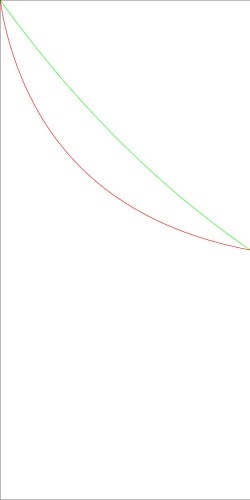
2. Let $\varepsilon>0$. Consider $m$ sets $F_i$ of measure $\epsilon$ with pairvise intersections of measure $\varepsilon^2$ but no triple intersections (they are easy to construct by induction when $m\varepsilon<1$). Then $X_i=\chi_{F_i}-\varepsilon$ are pairwise independent with mean $0$ and $E|X_i|^p=\varepsilon(1-\varepsilon)^p+(1-\varepsilon)\varepsilon^p$. On the other hand, $$ E\left|\sum_i X_i\right|^p= \\ m(\varepsilon-(m-1)\varepsilon^2)(1-m\varepsilon)^p+\frac{m(m-1)}2\varepsilon^2(2-m\varepsilon)^p \\ +\left(1-m\varepsilon+\frac{m(m-1)}2\varepsilon^2\right)(m\varepsilon)^p\,. $$ Considering the regime $\varepsilon\to 0$, $m\varepsilon\to x\in(0,1)$, we get $$ (x-x^2)(1-x)^p+\tfrac{x^2}2(2-x)^p+(1-x+\tfrac{x^2}2)x^p\le C_p x\,. $$ Thus, $$ C_p\ge (1-x)^{p+1}+\tfrac x2(2-x)^p+(1-x+\tfrac{x^2}2)x^{p-1} $$ for every $x\in(0,1)$.

The graph of the maximum of the RHS over $x\in(0,1)$ is below (in red) compared to $2^{2-p}$ (in green) but it is clear that for $x$ close to $0$ the RHS tends to a number close to $2$ when $p\to 1$ (the first and the third term will be about $1$ each), so $C_{1+}=2$.

Answer 2

$\newcommand{\C}{\mathbb C}\newcommand{\p}[2]{#1^{[#2]}}\newcommand{\ol}[1]{\overline{#1}}$This is to provide another presentation of the second part of fedja's very ingenious answer.

The main differences are the following: (i) this presentation is more detailed and (ii) notation is simplified -- everything is expressed explicitly in terms of $p$, the $X_i$'s, and $z\in\C$, without using the symbols $G_i,u_i,H,v$.

Theorem: Suppose that $p\in[1,2]$, $S:=\sum_i X_i$, $\sum_i:=\sum_{i=1}^n$, and $X_1,\dots,X_n$ are independent symmetric random variables (r.v.'s) with values in $\C$ (so that $-X_i$ has the same distribution as $X_i$, for each $i$). Then \begin{equation*} E|S|^p\le\sum_i E|X_i|^p. \tag{10}\label{10} \end{equation*}

Proof: Inequality \eqref{10} is obvious when $p=1$ or $p=2$. So, it makes sense to try to interpolate between these two cases for $p$.

First, some preliminaries. Without loss of generality (wlog) $p\in(1,2]$, so that one can define $q:=\frac p{p-1}$, and then $\frac1p+\frac1q=1$. If $E|S|^p=0$ or $E|X_i|^p=\infty$ for some $i$, then \eqref{10} is trivial. So, wlog $\|S\|_p:=(E|S|^p)^{1/p}>0$ and $E|X_i|^p<\infty$ for all $i$. By the power-means inequality, $|S|^p\le n^{p-1}\sum_i|X_i|^p$. So, by (symmetric) truncation of the $X_i$'s and dominated convergence, wlog the $X_i$'s are bounded. Also, wlog \begin{equation*} \sum_i E|X_i|^p=1. \tag{20}\label{20} \end{equation*}

For complex $x$ and $z$, let \begin{equation*} \p xz:=|x|^{z-1}x \end{equation*} if $x\ne0$, with $\p0z:=0$. For such $x$ and $z$,

• $\p xz$ is holomorphic in $z$;

• $|\p xz|=|x|^{\Re z}$;

• $\p xz$ is odd in $x$, that is, $\p{(-x)}z=-\p xz$;

• so, if $X$ is a symmetric $\C$-valued r.v., then the r.v. $\p Xz$ is symmetric as well.

Now, the construction: For $z\in\C$, let \begin{equation*} F(z):=E Y_z S_z, \end{equation*} where \begin{equation*} Y_z:=\p{\bar Y}{(1-z)q},\quad Y:=\frac{\p S{p-1}}{\|S\|_p^{p-1}},\quad S_z:=\sum_i\p{X_i}{pz}, \end{equation*} and $\;\bar{}\ $ denotes the complex conjugation. Then

• $F\colon\C\to\C$ is an entire function;

• If $z=\frac1p$, then $Y_z=\bar Y=\dfrac{\p{\bar S}{p-1}}{\|S\|_p^{p-1}}$ and $S_z=S$, so that \begin{equation*} F(\tfrac1p)=\|S\|_p. \tag{30}\label{30} \end{equation*}

• If $\Re z=1$, then $|Y_z|\in\{0,1\}$ and $|\p{X_i}{pz}|=|X_i|^p$, so that $|F(z)|\le E|S_z|\le\sum_i E|X_i|^p=1$ by \eqref{20}.

• If $\Re z=\frac12$, then $|Y_z|^2=|Y|^q=\Big(\dfrac{|S|^{p-1}}{\|S\|_p^{p-1}}\Big)^q=\dfrac{|S|^p}{\|S\|_p^p}$, $E|Y_z|^2=1$, and $E|S_z|^2=\sum_i E|\p{X_i}{pz}|^2=\sum_i E|X_i|^p=1$, since the $\p{X_i}{pz}$'s are pairwise independent symmetric r.v.'s and in view of \eqref{20}. So, by the Cauchy--Schwarz inequality, $|F(z)|\le1$ if $\Re z=\frac12$.

So, $|F|\le1$ on the boundary of the strip $T:=\{z\in\C\colon\Re z\in[\frac12,1]\}$. Also, the entire function $F$ is bounded on $T$, since the $X_i$'s are bounded.

So, by the Phragmén–Lindelöf principle, $|F|\le1$ on the entire strip $T$. Since $\frac1p\in T$, and in view of \eqref{30}, we conclude that $\|S\|_p\le1$, which is equivalent to \eqref{10}, in view of \eqref{20}. $\quad\Box$