Integer Points on an Elliptic Curve

Question

I am trying to find integer points $(x,y)$ on the elliptic curve $$y^2=x^3-4x+9$$ Is there an elementary way to calculate all the solutions?

I have brute-forced solutions for $(x,y)$ under $1000$ and only $(2,3), (7,18), (11,36)$ seem to work. Does someone have a theoretical way of checking for all the solutions, or otherwise a Sage code would be appreciated?

Answer 1

The sage code is an one-liner:

EllipticCurve(QQ, [-4, 9]).integral_points(both_signs=True, verbose=True)

This gives some few details on the computations and lists in each pair (or two-torsion point) $\pm P$ of a point $P$ all possibilities. Here is the output, manually rearranged:

Using mw_basis  [(0 : 3 : 1), (2 : -3 : 1)]
e1,e2,e3:  1.35326397724897 - 1.22228072731230*I 
           1.35326397724897 + 1.22228072731230*I
          -2.70652795449793

Minimal and maximal eigenvalues of height pairing matrix: 
    0.456823765285265,
    1.04856634073590

x-coords of points on non-compact component with  -2 <=x<= 5
[-2, 0, 2]
starting search of remaining points using coefficient bound 6 and |x| bound 4.33701332419786e16

x-coords of extra integral points:
[-2, 0, 2, 7, 11, 646]
Total number of integral points: 12
[(-2 : -3 : 1),
 (-2 : 3 : 1),
 (0 : -3 : 1),
 (0 : 3 : 1),
 (2 : -3 : 1),
 (2 : 3 : 1),
 (7 : -18 : 1),
 (7 : 18 : 1),
 (11 : -36 : 1),
 (11 : 36 : 1),
 (646 : -16419 : 1),
 (646 : 16419 : 1)]

It is not easy to obtain the integral points by elementary means. The integral points are specific to the chosen Weierstraß model, the algebraic object (the elliptic curve) is only "living in background".

For the elliptic curve, we have a lot of special data already computed:

The LMFDB $\bbox[yellow]{\underline{7724a1}}$ label

---

---

To have an image of what is behind the wheels, i am trying to go into detail. I've learned about this way to attack the problem from

[Z] Don Zagier, Large integral points on elliptic curves,

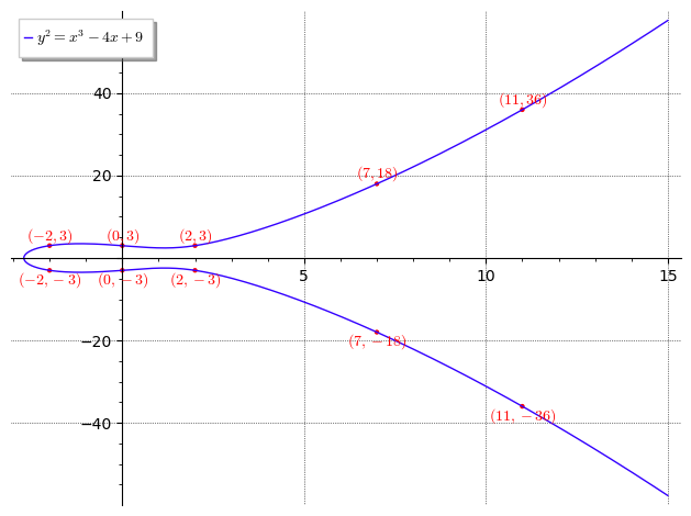
here Method 3 from [Z] applies only, since our curve $E$, $$ \tag{*} E\ :\ y^2 = x^3 -4x+9 \ , $$ does not have any rational torsion points. The group $(E(\Bbb Q),+)$ is a subgroup of $(E(\Bbb R),+)$, and a raw picture of the set $E(\Bbb R)$ is as follows:

p = E.plot(xmin=-15, xmax=+15, color=hue(0.7)
           , legend_label='$y^2 = x^3 - 4x + 9$', gridlines=True)
for P in E.integral_points(both_signs=True):
    if P.xy()[0] < 20:
        p += point(P.xy(), color='red')
        p += text(f'${P.xy()}$', P.xy()
                  , vertical_alignment='bottom' if P.xy()[1] > 0 else 'top'
                  , color='red')
p.show()

Consider the map: $$ \begin{aligned} \varphi\ &:\ E(\Bbb R)\to \Bbb R/\Bbb Z=:\Bbb T\ ,\\ \varphi(\xi,\pm \eta) &=\pm\frac 1\Omega\int_\xi^\infty\frac{dx}{\sqrt{f(x)}} \text{ modulo one,} \qquad\text{ where the signs correspond, and }\eta>0\ ,\\ \Omega &= 2\int_\gamma^\infty \frac{dx}{\sqrt{f(x)}} =2(\text{real period as recorded in LMFDB}) \approx 6.4590511833\dots \ ,\\ f(x) &= x^3 -4x+9\ ,\\ \gamma &= (\text{the only real root of the polynomial $f$}) \approx -2.70652795449793\dots \end{aligned} $$ (This explains some of the ingredients in the verbose information of sage above.)

The implemented algorithm uses now the knowledge of the generators for $E(\Bbb Q)$, which are (in some choice) $$ P=(0,3)\ ,\qquad Q=(2,-3)\ , $$ and then computes $\phi(P),\phi(Q)$. Assume there is some $R=(\xi,\eta)$ with integral components and "big" $\xi$-value, say $\xi>576=24^2$, and positive $\eta$. (Up to $576$ the brute force search is quickly done. And we a posteriori know there is such a point $R$ with $\xi>576$.) Then from the estimation

$\displaystyle x^3 -4x+9 \ge \left(1-\frac 1{50\,001}\right)x^3$ for $x\ge 574$,

we obtain $0<\phi(R)<\frac 1{\Omega}\int_{576}^\infty\frac {dx}{\sqrt{\frac{50\,000}{50\,001}}x^{3/2}}=\frac 1\Omega\cdot 2\cdot \sqrt{\frac{50\,000}{50\,001}}\cdot \frac 1{24}<0.013$ .

Then $R$ is a linear combination of $P,Q$, so $\varphi(R)$ is a corresponding linear combination of $\varphi(P), \varphi(Q)$. This is enough in practice to find integral points, we can theoretically say something about the bound, but still there is no proof. In this case, we can compute, first in a lazy, but explicit manner in sage (exactly as defined):

E = EllipticCurve(QQ, [-4, 9])
Omega = E.period_lattice().gens()[0] * 2

def phi(P):
    Px, Py = P.xy()
    sig = 1 if Py >=0 else -1 
    ni = numerical_integral( 1/sqrt(x^3 - 4*x +9), Px, oo)[0] * sig / Omega
    return ni - floor(ni)

P, Q = E.point((0, 3)), E.point((2, -3))
print(f"phi(P) ~ {phi(P)}")
print(f"phi(Q) ~ {phi(Q)}")

giving:

phi(P) ~ 0.341387000959375
phi(Q) ~ 0.776401416110533

then in pari/gp to have with higher precision the "same", we invoke ellpointtoz (for $-P$ instead of $P$ for the match)):

e = ellinit([-4, 9]);
g = e.omega[1];    // this is Omega/2
Omega = 2*g;
printf("Omega = %f", Omega)

P = [0, 3];
Q = [2, -3];

phiP = ellpointtoz(e, ellmul(e, P, -1)) / g
phiQ = ellpointtoz(e, ellmul(e, Q, -1)) / g

printf("phi(P) ~ %.80f", phiP)
printf("phi(Q) ~ %.80f", phiQ)

which gives:

phi(P) ~ 0.34138700095937692988380730758324050359907397748923935530998564831798527778370184
phi(Q) ~ 0.77640141611076055816015918015941761203541405951095543054592853694723627171494220

We search now for linear combinations of (the numerical values of) $\varphi(P),\varphi(Q)$ which are close to an integer, closer than $0.013$. For instance $$ \varphi(P)-3\varphi(Q) \approx -1.9878172473729047445966\dots $$ and the corresponding point is: $$ P-3Q=(646,16419)\ . $$

sage: P - 3*Q
(646 : 16419 : 1)

This is a way to find integral points of "high magnitude" on a given ($\Bbb Z$-model of an) elliptic curve. However, even in the case of a rank one elliptic curve, [Z] mentions that this is still far away from a proof. Combining methods mentioned in [Z], Method 2., one can say more for that specific case with a two-torsion point, and rank one, by combining height considerations and the Pell equation. But here, if we adjoin a root of $x^3-4x+9$ to the rationals, the resulted field has class number two, so we already leave an "elementary framework".

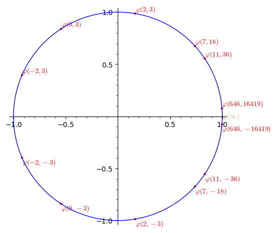
I have to conclude this part with a picture of the image of $\varphi$ for the known integral points:

(The "bigger" the integral point, the closer its $\varphi$-image gets to one.)

Used code:

p = circle((0, 0), 1)
p += point((1, 0), color='tan')
p += text('$\\varphi(\\infty)$', (1, 0), color='tan'
              , horizontal_alignment='left')

for P in E.integral_points(both_signs=True):
    valign = 'bottom' if P.xy()[1] > 0 else 'top'
    position = list(exp(2*pi*i*phi(P)).n())
    p += point(position, color='red')
    p += text(f'$\\varphi{P.xy()}$', position, color='red'
              , vertical_alignment=valign, horizontal_alignment='left')

p.show()

---

---

Can we do something by only elementary considerations?

(I'm afraid, not...)

We already have a list of integral points, the "biggest" one being $(646,\pm 16419)$ A first idea and try to eliminate other solutions then the found one would be by working modulo some (prime) numbers. But the curve has rank two over $\Bbb Q$, thus infinitely many rational points, and congruences tend to offer solutions. So there is more needed. This idea cannot effectively use the integrality hypothesis.

---

There are some ways to rewrite the equation with both sides having two or more factors, the first relation below is already in the comments, Chris Wuthrich mentioned it: $$ \begin{aligned} (y-3)(y+3) &=(x-2)x(x+2)\ ,\\ (y-18)(y+18) &= (x - 7)(x^2 + 7x + 45)\ ,\\ (y-36)(y+36) &= (x - 11)(x^2 + 11x + 117) \end{aligned} $$ Why is it hard to make a first step, e.g. starting from $(y-3)(y+3)=(x-2)x(x+2)$?

Let $(x,y)$ be a solution over $\Bbb Z$ of the given equation. Then $x-2$, $x$, $x+2$ are relatively prime, we take their factorizations, group then parts that appear in $(y-3)$, respectively $(y+3)$ for each. We obtain a scheme of the shape: $$ \begin{array}{|c|c|c|c|} \hline & x-2 & x & x+2 \\\hline y-3 & a & b & c \\\hline y+3 & d & e & f \\\hline \end{array} $$ Here, $a,b,c\ne 0$ are (odd and) relatively prime, and $d,e,f\ne 0$ are (odd and) relatively prime. In the corresponding system of equations $$ \left\{ \begin{aligned} x-2 &= ad\ ,\\ x &= be\ ,\\ x+2 &= cf\ ,\\[2mm] y-3 &= abc\ ,\\ y+3&=def\ , \end{aligned} \right. $$ any simple elimination of some of the variables does not really help. Comparing with [Z], second method, where a factorization worked, in that case the advantage was of having "two equal factors" on the $y$-side, and the number of variables resulted by using factorization arguments was much smaller, the half, it remained still a hard problem, but its relation to the Pell equation helped a lot.

But in this case this is not leading to a specific progress, at least i see no path to proceed.

Else, we may make some observations w.r.t. specific small primes. For instance, three divides one and exactly one of the factors $x,x+2,x-2$. So $3$ divides either $y+3$ or $y-3$, so it divides both. We can split into cases, but each such case is a new start.