Maximizing the expectation of a polynomial function of iid random variables

Question

Let $f \colon \mathbb R^N \to \mathbb R$ be a smooth function. Let $\mu$ be a probability measure on $[0,1]$ and $X_1, \ldots , X_N$ be i.i.d. random variables on $\mathbb R$.

Question 1. What is the maximum value of the expectation $$ \mathbb E[\vert f(X_1, \ldots , X_N) \vert] = \int_{\mathbb [0,1]^N} \vert f(x_1, \ldots , x_N) \vert d\mu(x_1) \ldots d\mu(x_N) $$ among all probability measures $\mu$ on $[0,1]$?

This question arises from this post and from this recent answer of Sangchul Lee which seem however tailored for specific functions $f$ and particularly for the case $N=2$.

I am very interested in the case $N\ge 3$; the function $f$ maybe be as smooth as needed (e.g. a polynomial). I have troubles in extending the (very elegant) variational approach of Sangchul Lee's to more variables, as no "bilinear form" is available.

After Nate Eldredge's comment, it is not restrictive to consider only a.c. measures. Furthermore, we can initially consider a somehow easier case, where $f$ is a polynomial (then maybe work by uniform approximation). In addition, thanks to a clever "random thought" due to Pierre PC (see comments below), we can start assuming symmetry of the integrand. All in all, the problem "boils down" to the following:

Question 1 (easier version): Maximize $$ \int_{[0,1]^N} p(x_1, \ldots, x_N) g(x_1) g(x_2) \ldots g(x_N) dx_1 dx_2 \ldots dx_N, $$ among functions $g \ge 0$ such that $\int_0^1 g(s)\, ds = 1$, being $p \in \mathbb R[x_1, \ldots , x_N]$ a symmetric polynomial (of constant sign on [0,1]?).

Can this be handled by the general Holder's inequality?

---

Since the general case seems too hard, let me propose a toy model we can begin with. To me, it seems the difficult point is not the integrand (in view of the comment above general reduction arguments should lead to a very simple form of it) but rather the fact that $N \ge 3$ (in comparison with S. Lee's approach, which is tailored for $N=2$).

So here we go:

Question 2. (baby version) What is the maximum value of the expectation $$ \mathbb E[|(X-Y)(Y-Z)(Z-X)|] = \int_{[0,1]^3} |(X-Y)(Y-Z)(Z-X)| d\mu(X) d\mu(Y)d\mu(Z) $$ among all probability measures $\mu$ on $[0,1]$?

Answer 1

We can in principle find the optimal first $n$ moments for a polynomial approximation of $f$. This reduces the problem to a truncated Hausdorff moment problem, for which solutions exist.

Let $f \colon [0,1]^d \to \mathbb{R}$ be a continuous function. Approximate $|f|$ with the multivariate Bernstein polynomials of order $n$ (writing $f_{k_1\cdots k_d} = f(k_1/n, \ldots k_d/n)$ for short),

$$|f_n|(x) = \sum_{k_1 \cdots k_d} |f_{k_1\cdots k_d}| \prod_{i=1}^{d} \binom{n}{k_i} \, x_i^{k_i} (1-x_i)^{n-k_i} \;.$$

Let $S_k = E[X^k (1-X)^{n-k}]$. The expectation of the approximant is then

$$E[|f_n|(X)] = \sum_{k_1 \cdots k_d} |f_{k_1\cdots k_d}| \prod_{i=1}^{d} \binom{n}{k_i} \, S_{k_i} \;,$$

which should be maximal. The value of $S_{k}$ is a linear combination on the first $n$ moments $M$ of the resulting distribution. Expanding

$$S_k = \sum_{r=0}^{n} \binom{n-k}{r-k} (-1)^{r-k} \, M_r \;,$$

the expectation in terms of the moments is

$$E[|f_n|(X)] = \sum_{k_1 \cdots k_d} \sum_{r_1 \cdots r_d} |f_{k_1\cdots k_d}| \prod_{i=1}^{d} \binom{n}{r_i} \binom{r_i}{k_i} (-1)^{r_i-k_i} \, M_{r_i} \;.$$

The problem is hence the constrained multilinear optimisation

$$ \begin{aligned} \max_{M_0 \cdots M_n} \;&\; \sum_{k_1 \cdots k_d} \sum_{r_1 \cdots r_d} |f_{k_1\cdots k_d}| \prod_{i=1}^{d} \binom{n}{r_i} \binom{r_i}{k_i} (-1)^{r_i-k_i} \, M_{r_i} \;, \\ \text{s.t.} \;&\; \sum_{r=0}^{n} \binom{n-k}{r-k} (-1)^{r-k} \, M_r \ge 0 \;, \\ &\; M_r \in [0,1] \;, \quad M_0 = 1 \;. \end{aligned} $$

To make the problem slightly more tractable, the relation between $S_k$ and $M_r$ can be inverted using the binomial partial sums,

$$M_r = \sum_{k=0}^{n} \binom{n-r}{k-r} \, S_k \;,$$

so that the optimisation becomes

$$ \begin{aligned} \max_{S_0 \cdots S_n} \;&\; \sum_{k_1 \cdots k_d} |f_{k_1\cdots k_d}| \prod_{i=1}^{d} \binom{n}{k_i} \, S_{k_i} \;, \\ \text{s.t.} \;&\; \sum_{k=0}^{n} \binom{n-r}{k-r} \, S_k \in [0,1] \;, \\ &\; \sum_{k=0}^{n} \binom{n}{k} \, S_k = 1 \;, \quad S_k \ge 0 \;. \end{aligned} $$

However, the first constraint is actually superfluous, as it is implied by the normalisation. Letting further $p_k = \binom{n}{k} S_k$, we have the optimisation problem in its most basic form,

$$ \begin{aligned} \max_{p_0 \cdots p_n} \;&\; \sum_{k_1 \cdots k_d} |f_{k_1\cdots k_d}| \prod_{i=1}^{d} p_{k_i} \;, \\ \text{s.t.} \;&\; \sum_{k=0}^{n} p_k = 1 \;, \quad p_k \ge 0 \;. \end{aligned} $$

which is simply the maximum expectation of the discretised function $|f_{k_1 \cdots k_d}|$ from the discrete distribution $p$.

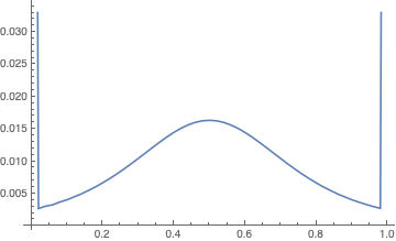
From a cursory Google search, multilinear optimisation appears difficult (but I have no idea, really). Nevertheless, it is a recipe for calculations: For the baby problem, I find (with $n = 50$) the expectation 0.0615760 and distribution $p$ as below.

Answer 2

Disclaimer: This is a bit too much "abstract nonsense" for me to really consider it a satisfying answer to the question, but on the other hand the question is so general that I'm not sure how much better one can do.

Let's write $E=[0,1]$ and $P(E)$ for probability measures on $E$. Let $f : E^n \to \mathbb{R}$ be bounded and measurable. (Actually, this all holds for an arbitrary Polish space $E$.) I claim that you can write

$$\sup_{\mu \in P(E)}\int_{E^n} f\,d\mu^n = \lim_{k\to\infty}\sup_{(x_1,\ldots,x_k) \in E^k}\frac{1}{k!}\sum_{\sigma \in S_k}f(x_{\sigma(1)},\ldots,x_{\sigma(n)}),$$

where $S_k$ is the set of permutations of $\{1,\ldots,k\}$, and $\mu^n$ is the $n$-fold product measure. As a sanity check, note that if $n=1$ then you can take $x_1=\ldots=x_k$ in the supremum to get $\sup f$. Not sure what to do with this for $n\ge 2$.

Proof: Fix $k \ge n$ for now. Then

$$\int_{E^n}f\,d\mu^n = \int_{E^k}f(x_1,\ldots,x_n)\,\mu^k(d(x_1,\ldots,x_k))$$

is a linear functional of $\mu^k$. The supremum of a linear functional over a convex set is the same as over its closed convex hull. Thus, if $C_k \subset P(E^k)$ denotes the closed (in total variation) convex hull of $\{\mu^k : \mu \in P(E)\}$, then

$$\sup_{\mu \in P(E)}\int_{E^n}f\,d\mu^n = \sup_{\nu \in C_k}\int_{E^k}f(x_1,\ldots,x_n)\,\nu(d(x_1,\ldots,x_k)).$$

Note that $C_k$ consists of all "mixtures of iid". Because De Finetti's theorem fails for finite exchangeable sequences, these "mixtures of iid" are not quite all exchangeable probability measures on $E^k$. However, if $P_e(E^k)$ denotes the set of exchangeable (invariant under permutations) probability measures on $E^k$, then a theorem of Diaconis-Freedman (Theorem 13 here) says that for each $\eta \in P_e(E^k)$ there exists $\nu \in C_k$ such that the projections $\eta|_n$ and $\nu|_n$ onto the first $n$ coordinates satisfy $\|\eta|_n-\nu|_n\|_{TV} \le n(n-1)/2k$, with $\|\cdot\|_{TV}$ denoting total variation. It follows that

$$\left|\sup_{\mu \in P(E)}\int_{E^n}f\,d\mu^n - \sup_{\eta \in P_e(E^k)}\int_{E^k}f(x_1,\ldots,x_n)\,\eta(d(x_1,\ldots,x_k))\right| \le \|f\|_\infty n(n-1)/2k.$$

Next, for a given $\eta$ we can average over all permutations of coordinates in $f$ without changing the value of the integral. That is,

$$\sup_{\eta \in P_e(E^k)}\int_{E^k}f(x_1,\ldots,x_n)\,\eta(d(x_1,\ldots,x_k)) = \sup_{\eta \in P_e(E^k)}\int_{E^k}\hat{f}_k\,d\eta,$$

where the function $\hat{f}_k : E^k \to \mathbb{R}$ is defined by

$$\hat{f}_k(x_1,\ldots,x_k) = \frac{1}{k!}\sum_{\sigma \in S_k}f(x_{\sigma(1)},\ldots,x_{\sigma(n)}).$$

We can then "un-symmetrize" the measures $\eta \in P_e(E^k)$ to reach a supremum over all probabilities on $E^k$:

$$\sup_{\eta \in P_e(E^k)}\int_{E^k}\hat{f}_k\,d\eta = \sup_{\eta \in P(E^k)}\int_{E^k}\hat{f}_k\,d\eta.$$

The right-hand side is simply $\sup \hat{f}_k$. Putting it all together gives

$$\sup_{\mu \in P(E)}\int_{E^n}f\,d\mu^n = \lim_{k\to\infty}\sup_{\eta \in P_e(E^k)}\int_{E^k}f(x_1,\ldots,x_n)\,\eta(d(x_1,\ldots,x_k)) = \lim_{k\to\infty}\sup \hat{f}_k,$$

which was the original claim above.

Answer 3

Suppose $\mu = \mu_{\max}$ is a (Borel) probability measure on $[0,1]$ for which the following integral is maximized: \begin{equation}\tag{1} \mathcal{I}(\mu) := \iiint |(y-x)(z-y)(z-x)| d\mu(x)d\mu(y)d\mu(z) \end{equation} Existence of $\mu_{\max}$ is relatively easy to prove. We will prove the following

Proposition: \begin{equation}\tag{2}\label{infinite} \limsup_{\epsilon \to 0} \frac{\mu_{\max}([0,\epsilon])}{\epsilon} = + \infty. \end{equation} That is, $\mu_{\max}$ has infinite density at $0$ and (by symmetry) also at $1$.

Here are some open questions:

• Is $\mu_{\max}$ atomic at $0$ and $1$?
• Is $\mu_{\max}$ absolutely continuous elsewhere?

First, we prove a

Lemma: If $X$ is a random variable with measure $d\mathbb{P}$ and cdf $F(x)$ satisfying $F(x)\le cx$ on $x\in [0,1]$, and $p=F(\epsilon)$, then

\begin{equation} \int_{[X \le \epsilon]} X d\mathbb{P} \ge \frac{p^2}{2c} \, . \end{equation}

Proof of Lemma: By a variant of the well-known identity for a non-negative random variable $X$: \begin{equation} \mathbb{E}(X) = \int_0^\infty (1-F(x))dx, \end{equation} we have \begin{align} \int_{[X\le \epsilon]} X d\mathbb{P} &= \int_0^\epsilon (p-F(x)) dx \\ &\ge \int_0^\epsilon \max(p-cx,0) dx \\ &\ge \int_0^{p/c} (p-cx) dx \\ &= \frac{p^2}{2c}. \end{align} This proves the Lemma.

The proof of the Proposition \eqref{infinite} is by contradiction. Let $\mu=\mu_{\max}$ and let $F(x) := \mu([0,x])$ be the cumulative distribution function. If the proposition does not hold, then there exists a finite $c \ge 1$ such that, for all $x\in [0,1]$, \begin{equation}\tag{3}\label{linear} F(x) \le cx . \end{equation} Note that $F(x)>0$ for every $x>0$, because if $F(x)=0$ for some $x>0$ then we can increase $I$ by replacing $\mu$ with $h_*\mu$, where $h$ is the affine map that sends $[x,1]$ onto $[0,1]$.

Let $X$, $Y$, $Z$ be independent random variables distributed according to $\mu$; let $\mathbb{P}$ denote the underlying probability. Fix a constant $\gamma \in (0,1)$ such that the following event $\Gamma$ has probability at least $1/2$: \begin{equation}\tag{4}\label{Gamma} \Gamma := \big[ Y>\gamma, \ Z>\gamma, \text{ and } |Y-Z|>\gamma \big]. \end{equation} Consider random variables $X_1 \le X_2 \le X_3$ obtained by ordering $X$, $Y$, $Z$; so $X_1 = \min(X,Y,Z)$, for instance. Fix a number $\epsilon$ in the range \begin{equation}\tag{5}\label{epsilon} 0 < \epsilon < \frac{\gamma^2}{12c}. \end{equation} Define random variables $\tilde{X}_1 \le \tilde{X}_2 \le \tilde{X}_3$ by: \begin{equation}\tag{6} \tilde X_i := \begin{cases} X_i &\text{if } X_i > \epsilon, \\ 0 &\text{otherwise.} \end{cases} \end{equation} Finally, define \begin{align} \Pi &:= (X_2-X_1)(X_3-X_1)(X_3-X_1) , \\ \tilde \Pi &:= (\tilde X_2- \tilde X_1)(\tilde X_3- \tilde X_1)(\tilde X_3- \tilde X_1) . \tag{7} \end{align} We claim that: \begin{equation}\tag{8}\label{mainclaim} \mathbb{E}(\Pi) < \mathbb{E}(\tilde \Pi) . \end{equation} This means that $\mathcal{I}(\mu) < \mathcal{I}(\nu)$, where $\nu$ is the probability measure obtained from $\mu$ by crunching all the mass of the interval $[0,\epsilon]$ on the point $0$. So the claim \eqref{mainclaim} implies that $\mu$ is not a maximizer, and therefore it is sufficient to prove it in order to conclude \eqref{infinite}.

Note that $\tilde \Pi = \Pi$ whenever $X_1 > \epsilon$, and so: \begin{equation}\tag{9} \mathbb{E}(\tilde \Pi - \Pi) = \int_{[X_1 \le \epsilon]} (\tilde \Pi - \Pi) d\mathbb{P} . \end{equation} On the other hand, $X_2 \le \epsilon$ implies $\tilde \Pi = 0$, so: \begin{equation}\tag{10}\label{difference} \mathbb{E}(\tilde \Pi - \Pi) = - \int_{[X_2 \le \epsilon]} \Pi d\mathbb{P} + \int_{[X_1 \le \epsilon < X_2]} (\tilde \Pi - \Pi) d\mathbb{P} =: -I_1 + I_2 . \end{equation} Let us estimate the integrals $I_1$ and $I_2$.

Let \begin{equation}\tag{11}\label{p} p := \mu([0,\epsilon]) = \mathbb{P}[X\le \epsilon]. \end{equation} Then: \begin{align} \mathbb{P}[X_2\le \epsilon] &= \mathbb{P}[X_2\le \epsilon < X_3] + \mathbb{P}[X_3\le \epsilon] \\ &= 3p^2(1-p) + p^3 \\ &\le 3p^2 \, . \tag{12} \end{align} On $[X_2 \le \epsilon]$ we have $\Pi \le X_2-X_1 \le X_2 \le \epsilon$. Therefore we obtain the bound \begin{equation}\tag{13}\label{I1} I_1 \le 3 \epsilon p^2 . \end{equation}

Let us estimate $I_2 = \int_{[X_1 \le \epsilon < X_2]} (\tilde \Pi - \Pi) d\mathbb{P}$ from below. Note that the integrand is non-negative, and so \begin{equation}\tag{14} I_2 \ge \int_{G} (\tilde \Pi - \Pi) d\mathbb{P} \end{equation} for any measurable set $G \subseteq [X_1 \le \epsilon < X_2]$. We choose $G:= [X \le \epsilon] \cap \Gamma$, where $\Gamma$ is as in \eqref{Gamma}. Over $G$ we have: \begin{align} \tilde \Pi - \Pi &= YZ |Y-Z| - (Y-X) (Z-X) |Y-Z| \\ &= X(Y + Z - X) |Y-Z| \\ &\ge \gamma^2 X.\tag{15} \end{align} Therefore: \begin{equation}\tag{16} I_2 \ge \int_{G} (\tilde \Pi - \Pi) d\mathbb{P} \ge \gamma^2 \int_{[X \le \epsilon] \cap \Gamma} X d\mathbb{P} = \gamma^2 \mathbb{P}(\Gamma) \int_{[X \le \epsilon]} X d\mathbb{P} \end{equation} (since the random variable $X$ is independent from the event $\Gamma$).

Then by the lemma, $I_2 \ge \gamma^2 p^2/4c$ and therefore: \begin{equation}\tag{17} \mathbb{E}(\tilde \Pi - \Pi) = I_2 - I_1 \ge \left(\frac{\gamma^2}{4c} - 3 \epsilon \right) p^2 > 0, \end{equation} by our choice of $\epsilon$. This proves the claim \eqref{mainclaim} and the Proposition.

Answer 4

We can attack the baby problem directly, as Jairo Bochi and I did jointly in the comments.

For instance, the distribution which is a mixture of:

• $3/5$ of a Bernoulli distribution with $p=1/2$
• $2/5$ of a Beta distribution with $\alpha=\beta=4$

yields an expectation equal to $503582/8204625$, or approximately $.0614$. This mixture of a discrete and a continuous distribution seems to be almost optimal.

Answer 5

Here is a complete and elementary solution for the Baby-squared problem, that is, the Baby Problem with the integrand squared. The idea is to reformulate the problem in terms of moments, and originates from @student's answer. By a linear change of coordinates, we can work on the interval $[-1,1]$ instead. The result becomes:

Proposition: For any Borel probability measure on $[-1,1]$, we have \begin{equation}\tag{1}\label{prop} \iiint (y-x)^2 (z-y)^2 (z-x)^2 \, d\mu(x)d\mu(y)d\mu(z) \le \frac{8}{9}. \end{equation} Equality holds if and only if \begin{equation}\tag{2}\label{three} \mu = \frac{\delta_{-1}+\delta_0+\delta_1}{3} . \end{equation}

Remark: As explained in other answers and comments, the maximizer $\mu$ for the original (un-squared) Baby Problem is certainly more complicated than \eqref{three}, and it seems to have a discrete and a continuous component.

Lemma: If $X$ is any random variable on $[0,1]$, then: \begin{equation}\tag{3} \mathbb{E}(X) \, \mathrm{Var}(X) \le \frac{4}{27} . \end{equation} Equality holds if and only if $X$ is Bernoulli with $\mathbb{P}[X=0] = 1/3$, $\mathbb{P}[X=1] = 2/3$.

Proof of the lemma: There should be a direct argument, but here is a somewhat informal proof. If $0<X<1$ with positive probability then we can deform the distribution of $X$ so that expectancy doesn't change and the variance increases. Therefore expectancy times variance can only be maximized if $X$ is Bernoulli taking values $0$ or $1$. Then the lemma becomes a Calculus exercise.

Proof of the proposition: Let $\mu$ be a Borel probability measure on $[-1,1]$. For each positive integer $n$, let $M_n := \int x^n \, d\mu(x)$ denote the $n$-th moment of $\mu$. Let $I$ denote the LHS of \eqref{prop}. Computation shows that: \begin{equation}\tag{4}\label{formula} I = 12 M_1 M_2 M_3 - 6 M_1^2 M_4 - 6 M_3^2 + 6 M_2 M_4 - 6 M_2^3. \end{equation} [Curiosity: the fact that the expression on the RHS is nonnegative is a well-known general property of moments; actually the RHS is $6$ times the determinant of the positive-semidefinite Hankel quadratic form $Q(u_0,u_1,u_2) := \int (u_0+u_1 x + u_2 x^2)^2 \, d\mu(x)$.] Note that: \begin{equation}\tag{5} 2 M_1 M_2 M_3 \le M_1^2 M_2^2 + M_3^2 \le M_1^2 M_4 + M_3^2 . \end{equation} This gives: \begin{equation}\tag{6}\label{nice} I \le 6 M_2 M_4 - 6 M_2^3. \end{equation}

Consider the probability measure $\hat{\mu}:=(\mu+r_* \mu)/2$ on $[-1,1]$, where $r(x) := -x$; this measure is symmetric around $0$ (in the sense that $r_* \hat{\mu} = \hat{\mu}$). The moments of $\hat{\mu}$ are: \begin{equation}\tag{7} \hat{M}_n = \begin{cases} M_n &\text{if $n$ is even,}\\ 0 &\text{if $n$ is odd.} \end{cases} \end{equation} Let $\hat{I}$ denotes integral on the LHS of \eqref{prop} with $\hat{\mu}$ in the place of $\mu$. Then inequality \eqref{nice} can be rewritten as: \begin{equation}\tag{8} I \le \hat{I} \, . \end{equation} Furthermore, it's easy to check that if $I = \hat{I}$ then $\mu$ is symmetric around $0$ or $I=0$.

Therefore we can assume that $\mu = \hat{\mu}$, that is, $\mu$ is symmetric around $0$. In this case, \begin{equation}\tag{9} I = 6 M_2 M_4 - 6 M_2^3 = 6 M_2 (M_4 - M_2^2) = 6 \mathbb{E}(X^2) \mathrm{Var}(X^2) \, , \end{equation} where $X$ is a random variable with distribution $\mu$. By the lemma, $I \le 8/9$, with equality if and only if $X^2$ is Bernoulli with $\mathbb{P}[X^2=0] = 1/3$ and $\mathbb{P}[X^2=1] = 2/3$. By symmetry, this means that $X$ is Bernoulli equidistributed on $\{-1,0,1\}$. The proposition is proved.