Intuition and/or visualisation of Itô integral/Itô's lemma

Question

Riemann-sums can e.g. be very intuitively visualized by rectangles that approximate the area under the curve. See e.g. Wikipedia:Riemann sum.

The Itô integral has due to the unbounded total variation but bounded quadratic variation an extra term (sometimes called Itô correction term). The standard intuition for this is a Taylor expansion, sometimes Jensen's inequality.

But normally there is more than one intuition for a mathematical phenomenon, e.g. in Thurston's paper, "On Proof and Progress in Mathematics", he gives seven different elementary ways of thinking about the derivative.

My question
Could you give me some other intuitions for the Itô integral (and/or Itô's lemma as the so called "chain rule of stochastic calculus"). The more the better and from different fields of mathematics to see the big picture and connections. I am esp. interested in new intuitions and intuitions that are not so well known.

Answer 1

I find the intuitive explanation in Paul Wilmott on Quantitative Finance particularly appealing.

Fix a small $h>0$. The stochastic integral $$\int_0^{h} f(W(t))\ dW(t)=\lim\limits_{N\to\infty}\sum\limits_{j=1}^{N} f\left(W(t_{j-1})\right)\left(W(t_{j})-W({t_{j-1}})\right),\quad t_j= h\frac{j}{N},$$ involves adding up an infinite number of random variables. Let's substitute every term $f\left(W(t_{j-1})\right)$ with its formal Taylor expansion. Then there are several contributions to the sum: those that are a sum of random variables and those that are a sum of the squares of random variables, and then there are higher-order terms.

Add up a large number of independent random variables and the Central Limit Theorem kicks in, the end result being a normally distributed random variable. Let's calculate its mean and standard deviation.

When we add up $N$ terms that are normal, each with a mean of $0$ and a standard deviation of $\sqrt{h/N}$, we end up with another normal, with a mean of $0$ and a standard deviation of $\sqrt{h}$. This is our $dW$. Notice how the $N$ disappears in the limit.

Now, if we add up the $N$ squares of the same normal terms then we get something which is normally distributed with a mean of $$N\left(\sqrt{\frac{h}{N}}\right)^2=h$$ and a standard deviation which is $h\sqrt{2/N}.$ This tends to zero as $N$ gets larger. In this limit we end up with, in a sense, our $dW^2(t)=dt$, because the randomness as measured by the standard deviation disappears leaving us just with the mean $dt$.

The higher-order terms have means and standard deviations that are too small, disappearing rapidly in the limit as $N\to\infty$.

Answer 2

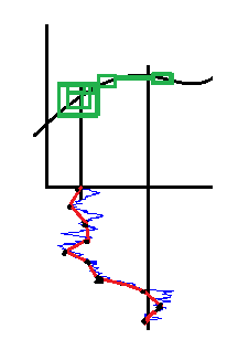
I know this thread is already two years old, but, while preparing for a path integration exam, I arrived at an intuitive picture that sheds some light on the origin of the extra term. The picture represents an integral of a smooth function with respect to a concrete realization of Brownian motion. The sum of the areas of the green rectangles represents the difference between Ito (using the left point of each interval) and "anti-Ito" (using the right point of each interval) for sampling of the Brownian motion represented by the red line. Finer sampling leads to smaller rectangles, but they overlap more and more (because Brownian motion is not monotonic), so even if the area occupied by them tends to zero, the sum of their areas does not. This suggests (only suggests -- it is an upper bound on the difference, not a lower bound) that there is a "room" for Ito and "anti-Ito" to differ in their values. Stratonovich can be expected to lie somewhere in between.

Look at the following image:

https://lh6.googleusercontent.com/-bEPzm01WyGk/T-WplGQAc3I/AAAAAAAAACQ/mZr-5p0VUrw/s317/integral-wrt-brownian-motion.png

                

Answer 3

I found this explanation somewhere and wrote it down in my personal notes. I will explain with an example that I think exemplify why Riemann-Stieltjes will provide the wrong answer.

First, let's remember how we can define the Riemann-Stieltjes integral below

\begin{equation}\int_0^t Z(x)dZ(x)=\lim_{n\rightarrow\infty}\sum_{k=1}^n(Z(t_k)-Z(t_{k-1}))Z(t_{k-1})\tag{*}\end{equation}

where $0=t_1<t_2<...<t_n=t$, when $n\rightarrow\infty$, $(t_k-t_{k-1})$ goes to zero and $Z(x)$ is continuous and has bounded variation. The Ito integral can be defined in the same way (assuming $Z(t)$ to be any Brownian Path). So, in this elementar definition there is not really any difference, it is just that each is dealing with different kind of functions. But the integration rules will be different.

We can rewrite the terms in the sum as:

$$\sum_{k=1}^n(Z(t_k)-Z(t_{k-1}))Z(t_{k-1})=\frac{1}{2}Z(t)^2-\frac{1}{2}\sum_{k=1}^n(Z(t_k)-Z(t_{k-1}))^2$$

To exemplify, let's assume now that $Z(x)=x$. We know how to solve the integral in this case, this is $0.5t^2$, as in the first term of RHS above. What happens with this function is that we can ignore the second term above, since it will go to zero (try partioning $[0,t]$ with $t_k=kt/n$, for example). This comes from the fact that $Z(x)=x$ has bounded variation.

Why can't we simple do this if $Z(t)$ is a Brownian Path? The problem here is that $\frac{1}{2}\sum_{k=1}^n(Z(t_k)-Z(t_{k-1}))^2$ won't go to zero when $n\rightarrow \infty$. In fact,

$$\lim_{n\rightarrow\infty}\frac{1}{2}\sum_{k=1}^n(Z(t_k)-Z(t_{k-1}))^2=t$$

This is so because we are considering infinite realizations of a normal variable with variance $t_k-t_{k-1}$ as $n$ goes to infinity. The Brownian Path limit above does not go to zero because it fails to satisfy bounded variation.

That is why, even though Ito and Riemann-Stieltjes integration depart from the same definition (*) the results are very different. If $Z(x)$ is a Brownian Motion we get:

$$\int_0^t Z(x)dZ(x)=\frac{1}{2}Z(t)^2-\frac{1}{2}t$$

While if $Z(x)$ is a continuous function with bounded variation we get

$$\int_0^t Z(x)dZ(x)=\frac{1}{2}Z(t)^2$$

Answer 4

Robert Anderson used nonstandard analysis to generate Brownian motion from a finite random walk obtained from coin tosses, where "finite" means indexed by an infinite, non-standard natural number. The corresponding random walk has bounded variation under a non-standard bound. One can then do everything in terms such an random walk, as has been done without rigorous justification before. The Itô-integral can be obtained from a Stiltjes-integral on the random walk, they differ only by an infinitesimal. An outline of the arguments can be found here. For the details, see:

MR0464380 (57 #4311) Anderson, Robert M. A non-standard representation for Brownian motion and Itô integration. Israel J. Math. 25 (1976), no. 1-2, 15--46.

Answer 5

One way to improve intuition is to work out a couple of

Discrete versions of Ito's lemma

1. Øksendal (6th edition) Example 3.1.9: almost surely, $$ B_t^2 - t = \int_0^t 2B_s dB_s $$

This has a discrete version which holds everywhere: let $X_n=\pm 1$ and $S_n=\sum_{i=1}^n X_i$, then $$ S^2_n-n = 2\sum_{i=0}^{n-1} S_i X_{i+1} $$ To verify just note that both sides increase by $2S_{n-1}X_n$ when going from $n-1$ to $n$.

2. Øksendal's exercise 4.2: $$ B_t^3 = \int_0^t 3B_s ds + \int_0^t 3B_s^2 dB_s $$

Here the discrete version is not a perfect analogue: $$ S_n^3 - S_n = 3\sum_{i=0}^{n-1} (S_i + S_i^2 X_{i+1}) $$ The extra term $S_n$ seems related to the fact that $(dB_t)^3 = 0$.

Answer 6

Consider the stochastic process

$$f(B_t)$$

where $B_t$ is standard Brownian motion (or the Wiener process) and $f$ is a twice-differentiable function.

Ito’s lemma states that

$$df = f'(B_t) dB_t + \frac{1}{2} f''(B_t) dt$$

The first term is recognizable from the chain rule in classical calculus, but why the second term? If $dB_t$ is truly infinitesimal, it doesn’t even seem possible that $df \neq f'(B_t) dB_t$.

To understand Ito’s lemma intuitively, think of $dB_t$ as a little stochastic variable, specifying $B_t$‘s change during the next $dt$.

$$dB_t = B_t - B_{t+dt} \sim N(0,dt)$$

This models Brownian motion (or the Wiener process) completely. Now $df$ should be a little stochastic variable too, modeling the stochastic process $f(B_t)$.

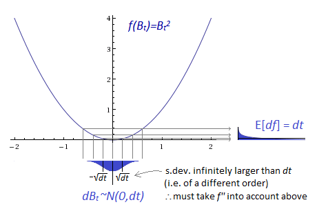
The picture at the start considers an example $f(B_t)$ where $f'(B_t)=0$, thereby suppressing the “intuitive” or classical term in Ito’s lemma. The reason why $df>0$ in that picture is the reason why that “non-intuitive” term is needed.

Loosely speaking, wherever $f$ has curvature, $dB_t$ will diffuse around that curvature sufficiently to influence the expected result on the order of $dt$. (The specific example in the picture makes this trivial, as $f(\sqrt{t}) = t$.)

Why doesn’t $dB_t$ dominate away $(dB_t)^2$ (i.e. $dt$ )? Because $E[(dB_t)^2]$ does not come from $(E[dB_t])^2$ as happens with classical differentials. The strong law of large numbers implies that a stochastic differential’s expected value pushes its integral on a faster order than its deviation does.

Answer 7

Here is my two cents on an intuitive explanation of the Ito integral:

The Ito integral is $\int_S^T f(t,w) dB(t,w)$

We can thing of $B(t,w)$, the Brownian motion as the actual price (with mean subtracted) and $f(t,w)$ is a random trading action and its gain on the observable prices. As a result, $f(t,w)$ is $F_t$ adaptive, i.e., it can be dependent only on the history of the prices not future prices. Then, the Ito integration is the total gain from $S$ to $T$ using random trading action+gain $f(t,w)$.

Answer 8

Yet another angle on this:

Normally, when we integrate a deterministic function, time always moves forward. Thus, in a question like $\int_0^t t dt$ or $\int_0^t t^2 dt$ t always moves forward and the t's are fully determined. By that I mean that we know (in the second case) at all time what the value of $t^2$ is - at 2 it has the value 4, at 3 it has the value 9, etc. We are doing a Riemann integral to get the area under the curve. $t$ is deterministic.

On the other hand, look at $\int_0^t W_t dW_t$. Here $W_t$ is not deterministic. But, for small $\Delta t$, $W_t$ changes by $dW_t$. But that means $W_t$ 'covaries' with $dW_t$. Now, if $dW_t$ is positive then $W_t$ goes up. But, if $dW_t$ is negative $W_t$ goes down. In both cases $W_t dW_t$ is positive and grows with time.

Thus, something like $\int_0^t W_t dW_t$ 'grows faster' than the deterministic $\int_0^t t dt$ as there is this positive addition each small $dt$. That is where the additional term comes in.

Answer 9

Suppose you ask a physicist, if a particle is at x = t^2. Now you ask him where the particle is an arbitrarily small time just before t = 1.

Physicists always just do a Taylor expansion around the point t = 1, and then say we can ignore second order terms. Thus, dx/dt = 2t, and we know at t = 1 the particle is at x = 1. So, the logic goes, if you are a small z away from t = 1, the particle is at 1 + 2z.

That is the deterministic rule. The problem for the stochastic world is that the same logic does not hold. If you are arbitrarily close to x = 1 (loosely speaking) at t = 1 - z, I believe the challenge is that P(X will not move very far in the tiny time left) does not drop off as quickly as second order Taylor terms owing to the variation of a stochastic process, so it can't be ignored. The Ito formula adjusts for this little oddity.

Answer 10

I like to interpret Ito Integral as the outcome of a gambling strategy (which fits in well with the fundamental property of the Integral: i.e. that it is forward-looking). In general, a stochastic Integral can be written as:

$$I_t:=\int_{h=0}^{h=t}Y_hdX_h=\lim_{n \to\infty}\sum_{h=0}^{n-1}Y_h\left(X_{h+1}-X_h\right)$$

Above, the limit is in probability, $X_t$ is some stochastic process (doesn't necessarily need to be a Standard Wiener Process) and $Y_t$ is a square-integrable process (obviously, doesn't need to be stochastic).

I interpret the integrator $X_t$ as the outcome of the gambling game, whilst the integrand $Y_t$ is the betting strategy (that is why the integrator is forward-looking by design: i.e. the bettor who places his bet at time $t$ is unable to see the outcome of the gambling game yet, which only gets realized at the next instance in time).

Simple illustrative example: let's suppose $H_t$ represents a coin-flip for each t (i.e. $H_t\in\left\{−1,1\right\}$ with probability 0.5, $H_0:=0$, $X_t:=\sum_{i=0}^{i=t}H_i$) and $Y_t=1$. Then a "discrete stochastic integral" could be defined as: $$I_{t=10}=\sum_{h=0}^{9}1\left(X_{h+1}-X_h\right)$$

This quantity computes the outcome of a gambling game after 10 rounds of betting, where each round the bettor bets consistently 1 unit of currency, and can either win or lose the amount he / she bets (obviously the above is a finite sum, it's just for illustrative purpose to build up the intuition).

Moving on, taking $X_t=W_t$ and $Y_t=W_t$, I interpret the Ito integral:

$$I_t:=\int_{h=0}^{h=t}W_hdW_h=\lim_{n \to\infty}\sum_{h=0}^{n-1}W_h\left(W_{h+1}-W_h\right)$$

as the outcome of a betting game, where initially the bettor bets $W_0:=0$, but each subsequent moment in time, the bettor bets the realized sum (up to that point in time) of Brownian increments $W_{h+1}−W_h$. These Brownian increments are at the same time the gambling game pay-off (so the game pays the bettor's last bet multiplied by the next Brownian increment realization).

In continuous time, the bettor constantly adjusts his or her bet to the "current" level of the Brownian motion $W_t$, which acts as the integrator: i.e. the betting game pays the realized Brownian $W_t$ at each moment in time multiplied by the bettor's bet corresponding to the last observed realization of $W_t$.

Finally, if the integrator is some stock price process $S_t$ instead of $W_t$, and $Y_t$ is the number of stocks held (could be simply a constant, deterministic quantity), then I interpret the corresponding Stochastic Integral $I_t:=\int_{h=0}^{h=t}ydS_h$ as the profit or loss of that stock portfolio over time.

(the answer above is taken from a similar answer I gave a while ago to a different question in Quant SE).

Answer 11

I would like to add another, not so well known, intuition: it is quite simple to demonstrate Ito's correction term in a binomial tree.

Details can be found in my paper (p. 8-10):
von Jouanne-Diedrich, Holger: Ito, Stratonovich and Friends (April 21, 2017)

Abstract
This exposition should provide you with the bigger picture of stochastic calculus, especially stochastic integrals. It heuristically and pedagogically develops key concepts and intuitions of one of the most important fields of applied mathematics today, namely quantitative finance. It demystifies ideas that a normally either too starkly dumbed down or hidden under highly technical details, so this text tries to fill a missing link in the literature where there seems to be no middle ground as of today. Additionally, the paper gives two results which cannot (to the best of my knowledge) readily be found in the classical literature: an illustration of the Ito correction term within binomial trees and a Taylor expansion for the Stratonovich integral.

Here I only give a summary of the general idea:

We start with a simple binomial tree with $n$ steps and $p=\frac{1}{2}$. Then we transform this tree with a convex function, e.g. with the quadratic function.

After that we compare the expected value of this transformed tree with the square of the expected value of the original tree - the difference is Ito's correction term.

All of this leads to a well-known identity: $$\mathbb{E}[X^2]=\mathbb{E}[X]^2+Var[X]$$

So in this case the variance can be interpreted as Ito's correction term - a nice correspondence to the well known $\frac{1}{2}\sigma^2$-term in the mean of the log-normal distribution.