Here is a family of alternatives. Let us identify the unit circle $C$ with the interval $[0,2\pi)$. For any two points $a$ and $b$ on the circle, consider the circular distance
\begin{equation*}
d(a,b):=\min(|a-b|,2\pi-|a-b|);
\end{equation*}
this is the geodesic (shortest) distance on the circle.
For any real $p\ne0$, any $J\subseteq[N]:=\{1,\dots,N\}$, and any point $a\in C$, let
\begin{equation*}
d_p(a,A_J):=\Big(\sum_{j\in J}d(a,a_j)^p\Big)^{1/p},
\end{equation*}
where
$A_J:=\{a_j\colon j\in J\}$, so that $d_p(a,A_J)$ is an "$L^p$ summary distance" from $a$ to the subset $A_J$ of your data set.
Note that $d_p(a,A_J)\to\min_{j\in J}d(a,a_j)$ as $p\to-\infty$ and $d_p(a,A_J)\to\max_{j\in J}d(a,a_j)$ as $p\to\infty$, provided that $J\ne\emptyset$.
Let then $a_{p,J}$ be any minimizer of the distance $d_p(a,A_J)$ in $a\in C$, so that $d_p(a_{p,J},A_J)\le d_p(a,A_J)$ for all $a\in C$; we may call $a_J$ an $L^p$-average of the set $A_J$. If the data set is not well enough clustered, then this average may be not unique. However, if the circle were replaced by a straight line with the usual metric on it and if $p=2$, then the $L^p$-average would be unique and it would coincide with the usual arithmetic mean.
Anyhow, the minimal distance $d_p(a_J,A_J)$ is uniquely determined for each $J\subseteq[N]$.
Now take a real $q$ and re-enumerate your data points $a_i$ in $[0,2\pi)$ so that
\begin{equation*}
d_q(a_1,A_{[N]\setminus\{1\}})\le d_q(a_2,A_{[N]\setminus\{2\}})\le \dots \le d_q(a_N,A_{[N]\setminus\{N\}}); \tag{1}
\end{equation*}
here one may want to use a (finite) negative $q$, so that, in accordance with a previous remark, $d_q(a_j,A_{[N]\setminus\{j\}})$ is somewhat similar to $\min_{i\in [N]\setminus\{j\}}d(a_j,a_i)$. Then, for some natural $n<N$, the points $a_{N-n+1},\dots,a_N$ are the $n$ data points with the largest "$L^q$ summary distance" to your data set, and so, these $n$ points may be considered the outliers; you may use the values of $d_q$ in (1) to choose your number $n$ of such outliers.
Letting then $J_n:=[N-n]=\{1,\dots,N-n\}$ and choosing a presumably positive real $p$, you will have $a_{p,J_n}$
as a "value which represents the truncated average of the data in the highest density around the circle", after the removal of $n$ "farthest outliers".
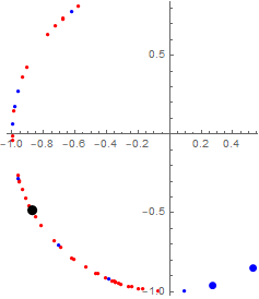
To illustrate this approach, a sample of size $40$ from the normal distribution with $\mu=0.6$ and $\sigma=0.1$ was simulated, and also another sample, of size $10$ from the normal distribution with the same $\mu=0.6$ and the greater $\sigma=0.15$. Then the two samples were combined into one, of size $50$; the fractional part of each of the $50$ values was taken; and all the results were multiplied by $2\pi$. This will be our set of the $a_i$'s. Then the approach described above was used with $q=-5$, $p=2$, and $n=2$ (outliers). The points on the unit circle obtained from the sample of size $40$ are the red points here in the picture; the blue points come from the more spread-out sample of size $10$; the two outliers (in this case they both come from the more spread-out, ``blue'' sample) are represented by the two blue points of a greater size; the big black point represents the truncated average $a_{p,J_n}$.

Remark: The subtle point in this approach is the recommendation that usually one should choose a finite negative value for $q$. Indeed, outliers may be understood, informally, as data points that lie far from the rest of data. So, one can try to measure the distances from potential outliers $a_j$ to the rest of the data as the minimum distance $\min_{i\in [N]\setminus\{j\}}d(a_j,a_i)$, which would correspond to $q=-\infty$, as mentioned before. But this choice of $q$ may be not the best sometimes. Indeed, usually outliers may be expected to be far away from one another. However, sometimes two outliers may turn out to be very close to each other, and then the minimum distance may not detect such outliers. To cover for such cases, one can use negative but finite values of $q$, to account also for the distances from the two (or more) such close-to-each-other outliers to the rest of the data. It seems to be a good idea to consider several negative values of $q$ and see how the outliers respond to such variation of the value of $q$.
In the first version of this answer, it was suggested to consider summary distances from potential outliers to subsets of the rest of the data of a certain size $m:=N-n<N$. This would take care of the problem of outliers very close to one another. However, then the volume of calculations would be much larger, on the order of $N^{n-1}$ times as large. Choosing a negative but finite $q$ seems to be a computationally much cheaper way to attain comparable quality of the results.

