Total absolute variation of brownian motion, with different sampling rates

Question

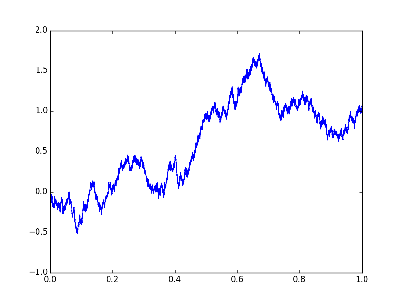
Let $(B_t)$ be a brownian motion on [0,1]. For the following, let $\omega$ be fixed.

Let's compute the total absolute variation when sampling period = $\delta$ is fixed:

$$V(\delta) = \sum_{i=0}^{N-1} |B_{t_{i+1}}(\omega) - B_{t_i}(\omega)|. $$

(i.e. $0 = t_0 < t_1 < t_2 < ... < t_N = 1$ with a constant step $\delta = t_{i+1} - t_i$ for all $i$)

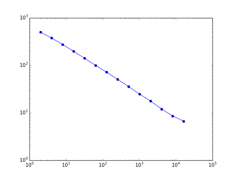
I noticed experimentally that:

$$ V(\delta) \sim c\ \delta^{-1/2}$$

It confirms the common-sense feeling that the smaller the sampling period (=the higher the sampling rate), the higher the total absolute variation.

Is it a well-known result? If so, where could I find a proof?

---

More generally, if for a process $X_t$ we have

$$ V(\delta) \sim c\ \delta^{-\kappa}$$

can we prove that $H = 1 - \kappa$ is the Hurst exponent of $X_t$ ?

It seems to work when $X_t$ is a $C^\infty$ function ($H=1$, $\kappa = 0$), it works for Brownian motion ($1/2$ for both), it also works for White noise ($H=0$, $\kappa = 1$).

---

Some Python code to show this:

# -*- coding: utf-8 -*-

import numpy as np
import matplotlib.pyplot as plt

# GENERATION OF BROWNIAN MOTION
X = 2 * np.random.binomial(1, 0.5, 2*1000*1000) - 1
cumsumX = np.cumsum(X)
n = 1000*1000
x = np.linspace(0, 1, num=1000*1000)
Y = 1/np.sqrt(n) * np.array([cumsumX[int(n*t)] for t in x])

plt.plot(x,Y)
plt.show()

# ABSOLUTE VARIATION FOR EACH DIFFERENT SAMPLING PERIOD
print('Sampling period, absolute variation')
SP = []
ABSVAR = []
for k in range(1,15):
    sp  = 2 ** k
    Z = Y[::sp]
    absvar=sum(abs(Z[1:]-Z[:-1]))
    SP.append(sp)
    ABSVAR.append(absvar)
    print sp, absvar

print('Coefficient:')
print((np.log(ABSVAR)[-1]-np.log(ABSVAR)[0])/(np.log(SP)[-1]-np.log(SP)[0]))

# LOGARITHMIC PLOT
plt.plot(SP, ABSVAR, marker='o')
plt.xscale('log')
plt.yscale('log')
plt.show()

Logarithmic plot of total absolute variation, in function of sampling period (both axis are log):

Answer 1

This is certainly well known. First of all, the variables $X_i=B_{t_{i+1}}-B_{t_i}$ are i.i.d. Gaussians with zero mean and variance $\delta$, which means that $|X_i|$ are i.i.d. with mean equal to $C_1\cdot\sqrt{\delta}$ and variance equal to $C_2\cdot\delta$. So, their sum has mean $C_1\delta^{-\frac12}$ and variance $C_2$. Moreover, by Chernoff's inequality, $$ \mathbb{P}\left(\left|\delta^\frac12\sum |X_i|-C_1\right|>\epsilon \right)\leq e^{-c(\epsilon)n} $$

You can now use Borel-Cantelli's lemma to deduce that almost surely, the total absolute variation of the sample path, rescaled by $\delta^\frac12$, converges to $C_1$.

Answer 2

Let $X$ be your list of $n$ elements representing the Brownian motion : $X_i$ is the position at the time $i$.

Let $Y=\{X_{i+1}-X_i\}$ be the list of differences of consecutive terms. As per your code, $Y$ follows a Gaussian distribution on $[-1,1]$.

Let $\delta$ be the sampling step.

Let $Z=\{X_0,X_{\delta},X_{2\delta},\dots\}$ be $X$ sampled.

We have $Z_{i+1}-Z_i=\displaystyle\sum_{j=0}^{\delta-1}Y_{i\delta+j}$

Thus $V(\delta)=\displaystyle\sum_{i=1}^{n/\delta}\left|\sum_{j=0}^{\delta-1}Y_{i\delta+j}\right|$.

which yields $\sigma(V(\delta))=\frac{n}\delta\frac{\sqrt\delta}2$

Let $c=\frac n2$, then $\boxed{\sigma(V(\delta))=\frac{c}{\sqrt\delta}}$.

Your program confirms this approach : we find $c\approx 55000=\frac n2,n=1000*1000$ as chosen in your program.