Consider independent random variables $Y_i$, $i>0$, such that $\mathbb{E}(Y_i)\approx \frac{1}{i}$ and $\text{Var}(Y_i)\approx \frac{1}{i^2}$, where $\approx$ means asymptotically equivalent up to a multiplicative constant. Define the partial sum $S_n=Y_1+\cdots+Y_n$. I am looking for a limit distribution of $S_n - \mathbb{E}(S_n)$. Note that Kolmogorov's three-series theorem applied to the centered random variables $Y_i - \mathbb{E}(Y_i)$ shows that an almost sure limit does exist.
A few directions that have revealed unsuccessful include:
- the traditional central limit theorem, since the $Y_i$'s are independent but not identically distributed
- triangular arrays CLT with i.d. variables, for the same reason
- Lindeberg-Feller type CLT, since the limit of $\text{Var}(S_n)$ is finite
- a direct characterization of the limit distribution by the characteristic function
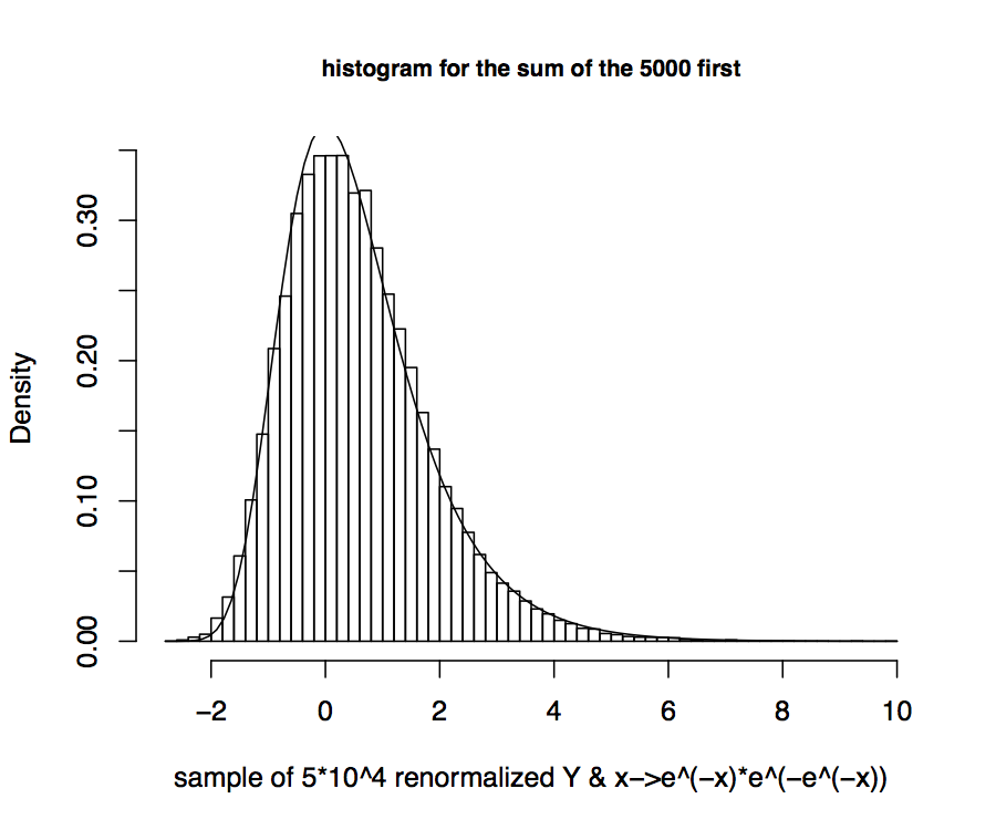
An example in Durrett's Probability book (Coupon collector's problem, Example 2.2.3. p 57) has the same kind of first two moments, and provides a Gumbel limit distribution. I tested this hypothesis numerically, and the adequation of the distribution of $S_n$ to a Gumbel distribution, for $n$ large, seems reasonably good. See the plot here, which represents an histogram for an independent sample of $S_n$ of size 50 000, with $n=5 000$, along with an adjusted Gumbel distribution:

I suspect some kind of Poisson limit behind this, as in Example 3.6.6. in Durrett's book, or as in Chapter 26 of Gnedenko and Kolmogorov's book (Limit distributions for sum of independent random variables). But I am not able to adapt the proofs to my setting.
Does anyone know if the Gumbel can occur as a limit distribution for such a sum? (for sure in extreme values theory, it represents the limit distribution of the maximum of an iid $n$-sample, but this is not the case here.) EDIT: The Gumbel is an Infinitely Divisible Distribution, and the way to prove it is to show that it is the limit distribution of $X_1+\ldots+X_n-\log(n)$, where $X_i\sim\text{Exp}(i)$.
Just to specify, the random variables are defined by $Y_j=-\log(1-V_j)$, where $V_j\sim\mbox{beta}(1-\sigma,\theta+j\sigma)$, $\sigma\in(0,1)$ and $\theta>-\sigma$. The reason for studying the sum $S_n$ is that it corresponds to $-\log$ of the tail sum, or rest, in a stick-breaking representation where the weights are defined by $\pi_i=V_i\prod_{j=1}^{i-1}(1-V_j)$.
