"Wild" solutions of the heat equation: how to graph them?

Question

It has long been known that the Cauchy initial-value problem for the classical heat equation on $\mathbb{R}$ (or $\mathbb{R}^n$) doesn't have unique solutions, without additional assumptions. In particular:

Theorem. There exist nontrivial $C^\infty$ functions $u : (-\epsilon, \epsilon) \times \mathbb{R} \to \mathbb{R}$ satisfying the heat equation $$\partial_t u - \partial_x^2 u = 0$$ with the initial condition $u(0,x) = 0$.

These functions must somehow represent disturbances arriving from infinity in finite time. They seem pretty weird to me and I think a picture would help with intuition.

I would like to see a graph of such a function. Where can I find one, or how can I generate it?

There are some explicit examples known. For instance, Rosenbloom and Widder [1] give the following: $$u(t,x) = \int_0^\infty e^{-y^{4/3}} y \cos(\sqrt{3} y^{4/3}) (e^{xy} \cos(xy + 2ty^2) + e^{-xy} \cos(xy-2ty^2))\,dy$$ as well as $$v(t,x) = \int_{a-i\infty}^{a+i\infty} e^{st + x\sqrt{s} - s^{2/3}}\,ds.$$ Unfortunately, the integrals are oscillatory and don't look so nice to approximate numerically.

Of course, there are various uniqueness theorems that give us qualitative information about what these nasty solutions must look like. Tychonoff's uniqueness theorem says $u(t,x)$ must grow faster than $e^{cx^2}$ near $x = \infty$, and Widder's theorem says that $u$ must be unbounded above and below for arbitrarily small $t$. But I'd really like to have an explicit picture to look at.

[1] Rosenbloom, P.C. and Widder, D.V. A temperature function which vanishes initially. American Mathematical Monthly 65(8):607-609, 1958.

Answer 1

Here's another plot (using Maple 17, and the first 21 terms) of the solution Carlo referred to.

Answer 2

Eq. 1.1 of this 1994 paper gives an explicit example in the form of a series expansion that seems tractable for numerical approximation. At least, I had no difficulty plotting a few terms of the series.

----Update-----

Thanks, Dirk, for the plot. If anyone would like to experiment a bit, you can input this line in Wolfram Alpha for a contour plot

ContourPlot[Sum[D[Exp[-1/t^2],{t,n}]*x^(2*n)/Factorial[2*n],{n,0,7}],{x,0,7},{t,0,7}]

(adjust {n,0,7} {x,0,7} {t,0,7} as desired for more terms in the sum or a different range of x and t)

I notice some curious features, like the oscillations for small t and large x.

Answer 3

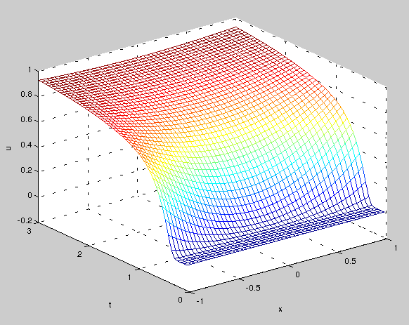
I know this is a late answer, but I think that the other answers posted so far completely fail to illustrate the wildness of the function in question, since they plot it on a domain where not much interesting happens. (Extending these computations to a larger and more interesting domain is not completely trivial, since one needs to use high precision and many more terms in order to get an accurate approximation. More about this below.)

So, again, this is Tychonoff's example, also treated in F. John's well-known textbook Partial Differential Equations (Fourth Edition), pp. 211–213: $$ u(x,t) = \sum_{n=0}^{\infty} \frac{g^{(n)}(t) \, x^{2n}}{(2n)!} $$ where $g(t) = \exp(-1/t^2)$ for $t>0$ and $g(t) = 0$ for $t \le 0$.

Obviously $u$ is even with respect to $x$, so it's enough to look at $x \ge 0$. Since $u$ is growing very quickly, I have plotted $\arctan u(x,t)$ instead of $u(x,t)$, so that the values stay in the range $(-\pi/2,\pi/2)$. Here are a few views of the graph, plotted on the grid $(x,t) \in [0,5] \times [0,1.5]$ using 400 terms in the sum (i.e., $\sum_{n=0}^{399}$) with spacing $\Delta x = 1/25$ and $\Delta t = 1/200$ between the sample points:

Here's the Mathematica code, in case someone wants to try it out. On my laptop, the computation took a little while, 15 minutes perhaps (I didn't keep track exactly).

numterms = 400;
digits = 50;
xdenom = 25; xmax = xdenom*5;
tdenom = 200; tmax = tdenom*3/2;
xmatrix = 
  Block[{Indeterminate = 1}, 
   N[Table[(i/xdenom)^(2 n), {i, 0, xmax}, {n, 0, numterms - 1}], 
    digits]];
tmatrix = {ConstantArray[0, numterms]}~Join~
  N[Table[CoefficientList[
       Series[Exp[-1/(j/tdenom + h)^2], {h, 0, numterms - 1}], h]*
      Table[Factorial[n]/Factorial[2 n], {n, 0, numterms - 1}], {j, 1,
       tmax}], digits];
umatrix = tmatrix . Transpose[xmatrix];
ListPlot3D[ArcTan[umatrix], 
 DataRange -> {{0, xmax/xdenom}, {0, tmax/tdenom}}, Mesh -> None, 
 PlotRange -> {-Pi/2, Pi/2}, AxesLabel -> {"x", "t", "arctan(u)"}]

Here's also an ordinary plot of $u$ itself, truncated at $\pm 5$:

ListPlot3D[umatrix, DataRange -> {{0, xmax/xdenom}, {0, tmax/tdenom}},
  Mesh -> None, PlotRange -> {-5, 5}, AxesLabel -> {"x", "t", "u"}]

The largest and smallest of the values computed at the gridpoints are $u(4.96,0.065) \approx 1.9 \times 10^8$ and $u(5,0.055) \approx -4.3 \times 10^8$.

To give an illustration of the complications, here is a plot of the base-10 logarithm of the absolute values of the first 400 terms in the sum defining $u(5,0.055)$, with blue/red dots for positive/negative terms:

c[x0_, t0_, n_] := 
 N[D[Exp[-1/t^2], {t, n}]*x^(2*n)/Factorial[2*n] /. {x -> x0, t -> t0}, 50]
coeffs = Table[c[5, 55/1000, k], {k, 0, 399}];
ListPlot[
 Map[Style[Log[10, Abs[#]], If[# > 0, Blue, Red]] &, coeffs], 
 PlotRange -> All]

These terms, which obviously span many different orders of magnitude, are computed using 50 digits of precision. The last one is less than $10^{-7}$, and after that they will keep on decreasing roughly geometrically (it seems), so 400 terms ought to be enough to give a good approximation to the true value of $u(x,t)$ at this point. When adding them all up, using Plus @@ coeffs, some precicion is lost, but Mathematica keeps track of this and gives its answer with as many digits as it thinks can be trusted, namely $-4.29528603477340289721804333 \times 10^8$.

As $x$ increases, so does the number of terms needed, at least for smallish values of $t$, where the function behaves wildly. For larger $t$, where $u \approx 1$, one doesn't need nearly as many terms, but my implementation is too stupid to take advantage of that. I'm not a numerical analyst, nor a Mathematica expert, so I'm sure there are many other things that could be done better too. Suggestions for improvements are welcome!

Answer 4

I made a MATLAB plot of a partial sum of the first seven terms of the series Carlo referred to. The series is $$ u(x,t) = \sum_{n=0}^\infty f^{(n)}(t)\frac{x^{2n}}{(2n)!} $$ where $$ f(t) = \begin{cases} \exp(-1/t^2) & t>0\\ 0 & t\leq 0 \end{cases} $$

The partial sum of the first seven terms looks like this:

It seems like the series is pretty much converged in this domain but I have the feeling that probably some interesting things may happen somewhere else.

One may say that this "wild" solution creeps out of zero so slowly that no one notices...