Cubic spline interpolation without a constant term

Question

Two main questions:

1. I am wondering if it is possible to construct a cubic spline that interpolates data WITHOUT a constant term $a$. That is, the polynomial takes the form $f(t) = bt + ct^2 + dt^3$, where $t$ is time.

2. Can this spline be used in global time. So rather than the traditional $b(t[i + 1]- t[i]) + c(t[i + 1]- t[i])^2 + d(t[i + 1] - t[i])^3$, we can just use $bt[i] + ct[i]^2 + dt[i]^3$.

I have tried different manipulations of the spline conditions to try and compensate for getting rid of the constant term, but have never been successful. If anyone has any insight into this I would greatly appreciate it!

Answer 1

It depends on what level of smoothness you require at your knots. The question only says that the spline has to interpolate data (= each piece must match the given values at the two knots that it connects). But when people say cubic spline, they usually mean that at each internal knot, the two pieces also have matching 1st and 2nd derivatives. But more generally you could require less smoothness, so let's consider three cases.

Suppose you have $n+1$ knots, thus $n$ pieces connecting them. (Since the question talks about "time", I am assuming that the final knot does not come back to the initial knot, that is, our spline does not form a closed loop.) You have $n-1$ internal knots (each between two adjacent pieces).

Without constant term, for each $i=1,\ldots,n$, the $i$th piece has 3 free parameters $b_i, c_i, d_i$, for a total of $3n$ parameters.

1. If no smoothness required: Each of the $n$ pieces must match both knots at its ends, so you have $2n$ conditions. Your $3n$ free parameters are ample and solutions should exist. But your "cubic spline" will look pretty funny because it will in general make corners at the knots.

2. If you require first derivatives to match at internal knots, that is $n-1$ more conditions. You now have $3n-1$ conditions, still less than your $3n$ free parameters, so it should be possible. Now your "cubic spline" has no corners at the knots (since first derivatives match), but its curvature will in general change abruptly (since second derivatives need not match). This may not be what you mean by "cubic spline".

3. If you require first and second derivative to match at the $n-1$ internal knots, you have $2n + 2(n-1) = 4n-2$ conditions, which is more than $3n$ (for $n>2$). You have more conditions than free parameters, so in general solutions will not exist. (They might exist in special cases.)

The usual definition has four parameters per piece, so $4n$ parameters total, which leaves 2 extra degrees of freedom even after matching first and second derivatives ($4n-2$ conditions). The usual way to use up these 2 dof is to impose that at the first and last knots, the second derivative vanishes (so called "natural" cubic spline).

---

Since we can at most require first-order smoothness (matching slopes), let us do that. A straightforward way is to set up $3n$ linear equations: $n$ for hitting left ends for each of the $n$ pieces; $n$ for hitting right ends, and $n-1$ for matching slopes. Oops, we only got $3n-1$ equations because there are only $n-1$ internal knots. For one more equation, let us arbitrarily fix the slope at first knot to some value $q$, for example $q=0$.

At the end of this answer there is very straightforward Matlab code illustrating how to do it. Optimized for simplicity, not efficiency or numerical stability.

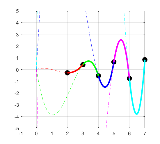
But let us first look visually at the interpolation of some small data (six knots). The solid lines show the cubic pieces over each interval.

Recall that the cubics do not have a constant term. So each cubic piece would hit the origin if you continued it to $x=0$, as illustrated with the dashed lines. I do not quite understand what real-world situation would call for such a requirement, and it causes the cubics to swing wildly; wilder towards the right end.

So in the end my answer is: Yes, it is possible, but why?

% Example data
x = [2 3 4 5 6 7];
y = sin(3*x);
n = length(x)-1;      % number of intervals
q = 0;                % required slope at first knot

% Intervals are numbered 1 to n.
% For each interval i there are 3 parameters:
% p(i)     = b coefficient of i'th polynomial
% p(i+n)   = c coefficient of i'th polynomial
% p(i+2*n) = d coefficient of i'th polynomial

% Initialize the coefficient matrix and RHS vector.
A = zeros(3*n, 3*n);
rhs = zeros(3*n, 1);

% Require hitting left ends.
for i=1:n
    A(i, i)     = x(i);
    A(i, i+n)   = x(i)^2;
    A(i, i+2*n) = x(i)^3;
    rhs(i)      = y(i);
end

% Require hitting right ends.
for i=1:n
    A(i+n, i)     = x(i+1);
    A(i+n, i+n)   = x(i+1)^2;
    A(i+n, i+2*n) = x(i+1)^3;
    rhs(i+n)      = y(i+1);
end

% Require matching slopes.
for i=1:n-1
    % Left-side slope at i'th internal knot, positive coefficients
    A(i+2*n, i)     = 1;         % b
    A(i+2*n, i+n)   = 2*x(i+1);    % c
    A(i+2*n, i+2*n) = 3*x(i+1)^2;  % d
    % Right-side slope at i'th internal knot, negative coefficients
    A(i+2*n, i+1)     = -1;         % b
    A(i+2*n, i+1+n)   = -2*x(i+1);    % c
    A(i+2*n, i+1+2*n) = -3*x(i+1)^2;  % d
    % Slope difference must be zero
    rhs(i+2*n) = 0;
end

% Required slope at first knot.
A(3*n, 1)     = 1;
A(3*n, 1+n)   = 2*x(1);
A(3*n, 1+2*n) = 3*x(1)^2;
rhs(3*n)      = q;

% Now require A*p = rhs.
p = A\rhs;


%%%%%%%%%%%%%%%%%%%%%%%%%%%%%%%%%%%%%%%
% Visualization

% Plot knots
clf
plot(x,y,'ko','markerfacecolor','k','markersize',10);
hold on
grid on

% Plot pieces
cols = 'rgbmcy';
for i=1:n
    xx = linspace(x(i), x(i+1), 100);
    yy = p(i)*xx + p(i+n)*xx.^2 + p(i+2*n)*xx.^3;
    plot(xx,yy,[cols(i) '-'],'linewidth',3);
end

% Plot continuations to origin
for i=1:n
    xx = linspace(0,x(i), 300);
    yy = p(i)*xx + p(i+n)*xx.^2 + p(i+2*n)*xx.^3;
    plot(xx,yy,[cols(i) '--']);
end

set(gca,'ylim',[-5 5]);