$\newcommand{\si}{\sigma}\newcommand{\ep}{\varepsilon}\newcommand\E{\operatorname{\mathsf{E}}}\newcommand\Var{\operatorname{\mathsf{Var}}}\newcommand{\de}{\delta}$I think a meaning can be attached to your post as follows: You appear to confuse three related but quite different notions: (i) a random variable (r.v.), (ii) its distribution, and (iii) its pdf. (Unfortunately, many people do so.)
So, my guess at what you were trying to say is as follows: Let $X$ be a r.v. with values in $[a,b]$. Let $\mu:=\E X$ and $\si^2:=\Var X$.
Let $X_{\cdot,\cdots}$ with various indices $_{\cdot,\cdots}$ denote independent copies of $X$. Let $t:=\lambda\in(0,1)$.
At the first step, we take any $X_1$ and $X_2$ (which are, according to the above convention, two independent copies of $X$). We multiply the r.v.'s $X_1$ and $X_2$ (not their distributions or pdf's) by $t$ and $1-t$, respectively, to get the independent r.v.'s $tX_1$ and $(1-t)X_2$. The latter r.v.'s are added, to get the r.v.
\begin{equation}
S_1:=tX_1+(1-t)X_2,
\end{equation}
whose distribution is the convolution of the distributions of the r.v.'s $tX_1$ and $(1-t)X_2$.
At the second step, take any two independent copies of $S_1$, multiply them by $t$ and $1-t$, respectively, and add the latter two r.v.'s, to get a r.v. equal in distribution to the r.v.
\begin{equation}
S_2:=t(tX_1+(1-t)X_2)+(1-t)(tX_3+(1-t)X_4) \\
=t^2 X_1+t(1-t)X_2+(1-t)tX_3+(1-t)^2X_4;
\end{equation}
(in accordance with the indexing convention, the r.v.'s $X_1,X_2,X_3,X_4$ are independent copies of $X$).
Continuing so, after the $n$th step we get a r.v.
\begin{equation}
S_n:=\sum_{k=0}^n t^k(1-t)^{n-k}\sum_{i=1}^{\binom nk} X_{n,k,i}
\end{equation}
(in accordance with the indexing convention, the $X_{n,k,i}$'s are independent copies of $X$). This expression for $S_n$ can be checked by induction on $n$. (One can also use/check the following re-indexed expression for $S_n$:
\begin{equation}
\sum_{(\de_1,\dots,\de_n)\in\{0,1\}^n}X_{\de_1,\dots,\de_n}
\prod_{j=1}^n(t^{\de_j}(1-t)^{1-\de_j});
\end{equation}
imagine the corresponding binary tree.)
Now we have
\begin{equation}
\begin{aligned}
\E S_n&=\sum_{k=0}^n t^k(1-t)^{n-k}\sum_{i=1}^{\binom nk} \E X_{n,k,i} \\
&=\sum_{k=0}^n t^k(1-t)^{n-k}\binom nk \mu =\mu
\end{aligned}
\end{equation}
and
\begin{equation}
\begin{aligned}
\Var S_n&=\sum_{k=0}^n (t^k(1-t)^{n-k})^2 \sum_{i=1}^{\binom nk} \Var X_{n,k,i} \\
&=\sum_{k=0}^n (t^2)^k((1-t)^2)^{n-k}\binom nk \si^2 \\
&=q^n\si^2\to0
\end{aligned}
\end{equation}
(as $n\to\infty$), where $q:=t^2+(1-t)^2\in(0,1)$.
So, by Chebyshev's inequality, for any real $\ep>0$,
\begin{equation}
P(|S_n-\mu|>\ep)\le\frac{\Var S_n}{\ep^2}=\frac{q^n\si^2}{\ep^2}\to0.
\end{equation}
Thus, indeed $S_n\to\mu$ in probability.
Moreover, since
\begin{equation}
\sum_{n=1}^\infty P(|S_n-\mu|>\ep)\le\sum_{n=1}^\infty\frac{q^n\si^2}{\ep^2}<\infty
\end{equation}
for any real $\ep>0$, it follows by the Borel–Cantelli lemma that $S_n\to\mu$ almost surely.
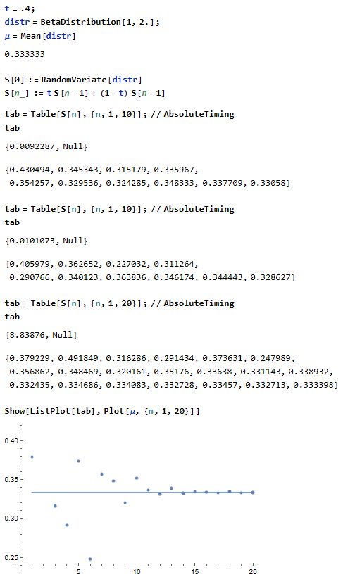
Below is the image of a Mathematica notebook illustrating the geometrically fast convergence of $S_n$ to the mean $\mu$. It takes Mathematica about 0.01 sec to simulate values of $S_1,\dots,S_{10}$ and about 9 sec to simulate values of $S_1,\dots,S_{20}$ (in the second case, we deal with a binary tree with $2^{20}\approx10^6$ leaves).


