Context: Q3 in How to understand the largest Lyapunov exponent?
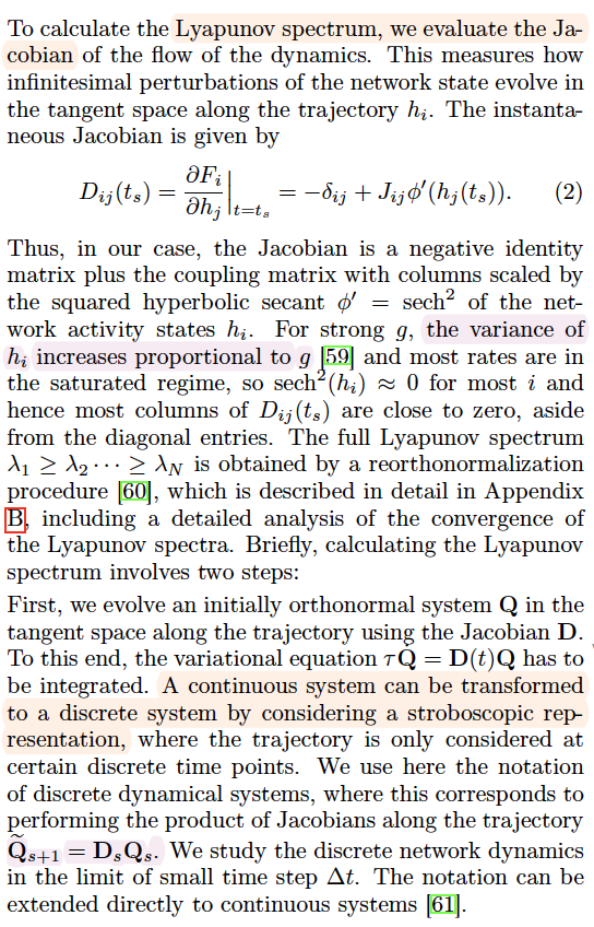
We know $g$ is proportional to (square root of) the variance of $J$'s every entry ($J_{ij}\sim \mathcal{N}(0,g^2/N)$).
Why is it also positively related to the variance of $h_i$.
In other words, why stronger coupling results in stronger neuronal signals, from a math perspective, in particular, for large systems?
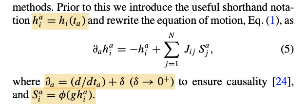
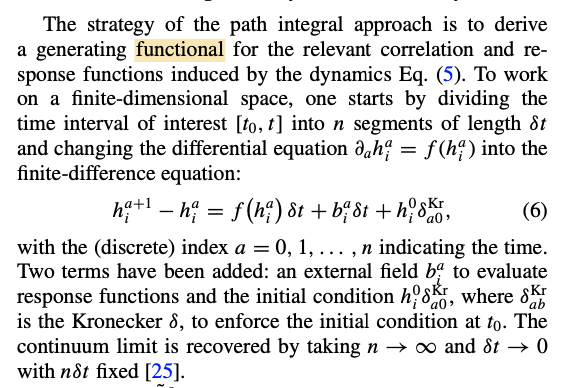
Clarification of notations in the paper (Crisanti, 2018):
Noteworthy details (Crisanti, 2018):
If the matrix $J_{ij}$ is symmetric, i.e., $J_{ji}=J_{ij}$, [...] The dynamics hence converges toward stable fixed points.
If the matrix is nonsymmetric, [...] a richer steady-state behavior emerges: besides fixed points, limit cycles and chaotic behavior are also possible.
The assumption of zero average implies that there is not a preferred type of synaptic connection... inhibitory ($N\overline J_{ij}<0$) or excitatory ($N\overline J_{ij}>0$).


General questions: The paper (Crisanti, 2018) is not easy for me. While I do not expect others to read the paper for me, how could I understand a paper like this? For example, what step should I follow, what prerequisite knowledge should I familiarize myself with?
Brief summary of topics and methods: The paper (Crisanti, 2018) uses some stochastic diff eq (SDE)/Ito (part of SD), functional, Fourier transform, etc.
The research seems to be within the domain of stochastic dynamics (SD) in statistical mechanics. The author here adopts a frequently used path integral method; while I am not familiar with the method, it seems to be about variational methods, which consider a functional (typically an integral; the author mentions 'action') and a small variation $\delta$, introduced to eq6 (Crisanti, 2018)(?) and resulting in a stochastic diff eq.
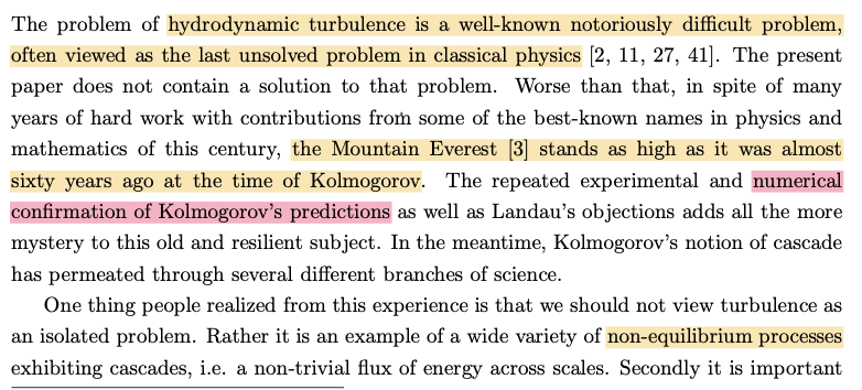
General background: The following is an excerpt from a paper (Weinan E, 2000) about stochastic PDEs in hydrodynamic chaos, which seems to be relevant to the above problem of chaos in neural networks.
Specific questions: When $J_{ij}$ is symmetric, there is an energy function (eq 3)(Crisanti, 2018), while when $J_{ij}$ is asymmetric, there is not, why? And why is the energy function in the form of eq3, and its relaxation in the form of eq2 (Crisanti, 2018)?
References:
A. Crisanti and H. Sompolinsky, Path integral approach to random neural networks, 2018 https://journals.aps.org/pre/abstract/10.1103/PhysRevE.98.062120 this is what is cited by the original paper (excerpted in the previous post) about $g$, $h_i$, and where most of the excerpts above come from.
H. Sompolinsky, A. Crisanti, and H. J. Sommers, Chaos in Random Neural Networks, 1988 https://journals.aps.org/prl/abstract/10.1103/PhysRevLett.61.259 this is a paper that gives solution to the nonlinear ODEs.
Weinan E, Stochastic PDEs in Turbulence Theory, 2000
NIPS 2006 Workshop on
Dynamical Systems, Stochastic Processes and Bayesian Inference www0.cs.ucl.ac.uk/staff/c.archambeau/dsb.htm
Path Integral Method for Estimation of Time Series www0.cs.ucl.ac.uk/staff/c.archambeau/accepts/restrepo.pdf


