Radial behavior of dynamical map $x_{n+1}=2x_ny_n$, $y_{n+1}=1-2x_n^2$

Question

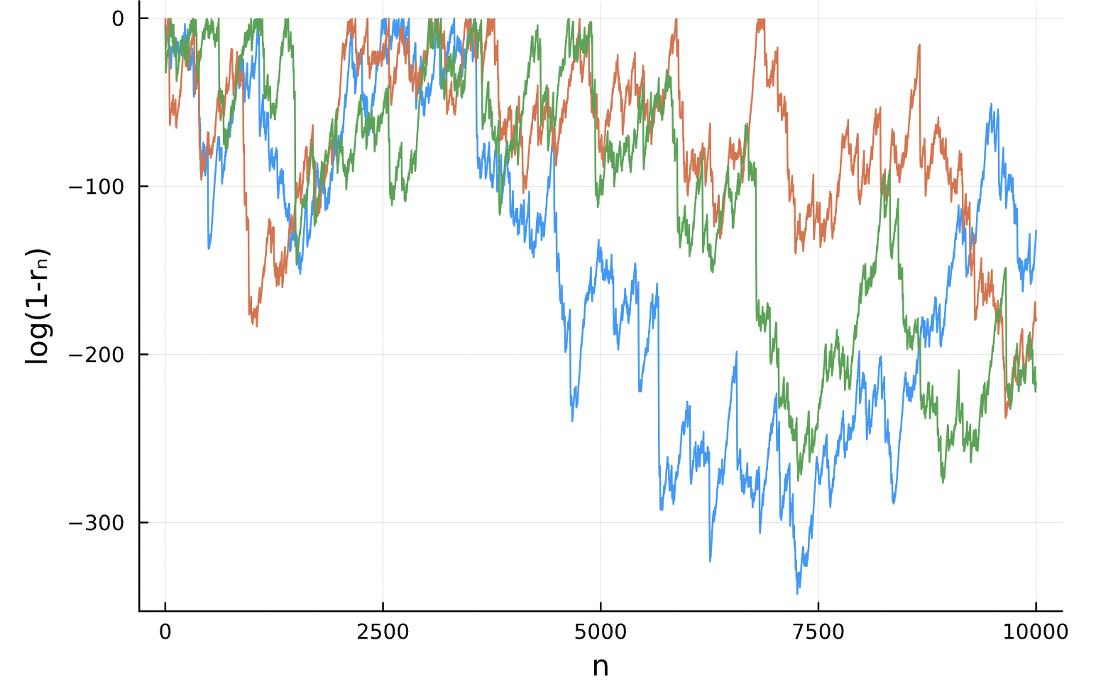
Consider the sequence in the unit disk $D=\{(x,y)\,|\,x^2+y^2\leq 1\}$ iteratively defined by the quadratic map $$\begin{aligned} x_{n+1}&=2x_ny_n\\y_{n+1}&=1-2x_n^2\end{aligned},$$ starting from some initial condition $(x_0,y_0)\in D$. It is easy to see that if the initial condition starts at the boundary $x_0^2+y_0^2=1$, then it stays in the boundary. My question is about initial conditions in the interior $x_0^2+y_0^2<1$. For these conditions, I am interested in the behavior of $r_n=\sqrt{x_n^2+y_n^2}$ for large $n$. Doing some numerics, one can see that the points approach the boundary, but not quite: there seems to be recurrences where $r_n$ goes away from $1$. See below a plot of $\log(1-r_n)$ for three random initial conditions $(x_0,y_0)\in D$.

Does $r_n\to 1$ eventually (i.e., $\log(1-r_n)\to -\infty$ in the plot below), or there are always recurrences where $\log(1-r_n)$ comes back close to $0$, for generic initial conditions? I suspect it is the latter (there will always be recurrences), but I do not know how I could prove this.

---

Update 2: From the great answers below (thanks!), it seems that there is enough evidence for generic non-convergence. I am interested in the proof of the following:

Conjecture: Let $E\subseteq D$ be the set of all initial conditions that converge to $\partial D$ under the dynamical system above. Then $E$ has (Lebesgue) measure zero.

---

Update 1: The Lyapunov exponents for almost all points at the boundary can be shown to equal $(\log(2),0)$. I am not sure if this prevents convergence $r_n\to 1$ for points in the interior (would appreciate input on this). Here is the computation:

One can convert the map into polar coordinates \begin{align} r_{n+1}^2&=1-4r_n^2(1-r_n^2)\cos(\theta_n)^2\\ \tan(\theta_{m+1})&=\left(\frac{1}{r_n^2}-1\right) \csc (2 \theta_n )-\cot (2 \theta_n ) \tag{1}\label{polareqs} \end{align}

Note that for conditions with $r_0=1$, we have $r_n=1$ for all $n$ and the angular map becomes the angle doubling map with an extra rotation: \begin{equation} \tag{2}\label{angularmap} \theta_{n+1}=2\theta_{n}-\tfrac{\pi}{2}\mod 2\pi. \end{equation}

The Jacobian at the boundary is \begin{equation} J(r=1,\theta)=\begin{pmatrix}\partial_r f_r& \partial_\theta f_r\\\partial_r f_\theta& \partial_\theta f_\theta \end{pmatrix}=\begin{pmatrix}4\cos(\theta)^2& 0 \\ -2\sin(2\theta) & 2 \end{pmatrix} \end{equation} where $r_{n+1}=f_r(r_n,\theta_n)$ and $\theta_{n+1}=f_\theta(r_n,\theta_n)$ according to Eq. \eqref{polareqs}.

The eigenvalues of $J(r=1,\theta_{n-1})\cdots J(r=1,\theta_1)J(r=1,\theta_0)$ are \begin{align} m_n^{(1)}&=2^n, \\ m_n^{(2)}&=4^n \cos(\theta_0)^2\cos(\theta_1)^2\cdots \cos(\theta_{n-1})^2 \end{align} Consequently, one Lyapunov exponent is $$\lambda^{(1)}=\lim_{n\to \infty}\frac{1}{n} \log(|m_n^{(1)}|)=\log(2).$$

The other Lyapunov exponent is given by $$\lambda^{(2)}=\lim_{n\to \infty}\frac{1}{n} \log(|m_n^{(2)}|)=\lim_{n\to \infty}\frac{1}{n}\sum_{j=0}^{n-1} \log(4\cos(\theta_j)^2).$$ This limit can be computed for almost every initial $\theta_0$ by assuming that the transformation Eq. \eqref{angularmap} is ergodic. I did not write down the proof, but this map is very similar to the angle doubling map, which is known to be ergodic. Ergodicity implies, by Birkhoff's ergodic theorem, that for almost all $\theta_0$, $$\lambda^{(2)}=\frac{1}{2\pi}\int_0^{2\pi}\log(4\cos(\theta)^2)d\theta=0.$$

Answer 1

OK, finally something about the measure. I'll put it into a separate answer again for readability. If the moderators frown upon such practice, they are welcome to merge in any way they find appropriate.

We shall show that for every Borel set $E\subset\mathbb D$, one has $$ \mu(E\setminus \cup_{j\ge 1} T^{-j}E)=0\,. $$ Here $Tz=z^2+1-|z|^2$ (I prefer to swap the coordinates, so that I can write $z=x+iy$) and $d\mu(z)=\frac{dA(z)}{1-|z|^2}$ is the invariant measure.

By the general mumbo-jumbo, that means that almost every point of $E$ returns to $E$ infinitely many times, from which it trivially follows that for almost every $z\in\mathbb D$, we have $\limsup_{n\to\infty} [1-|T^nz|^2]\ge 1-|z|^2>0$, answering the original question in the affirmative. I strongly suspect that this upper limit is at least some constant almost everywhere and, maybe, even $1$, but I cannot prove that much yet.

So, suppose that $E\setminus \cup_{j\ge 1} T^{-j}E$ contains a set $G$ of positive measure that is contained in the disk $\{\rho(z)\le \Delta\}$ where $\rho(z)=\frac 1{1-|z|^2}$. Then the sets $T^{-j}G$ are pairwise disjoint and have the same $\mu$-measure $\mu(G)$ each.

Let $S_{\pm}$ be the two right inverses to $T$, so $S_+(z)=\left(\frac y{\sqrt{2(1-x)}},\sqrt{\frac{1-x}2}\right)$, $S_-(z)=-S_+(z)$. We have $\rho(S_{\pm}z)=2(1-x)\rho(z)$ and $\mu(S_{\pm}E)=\frac 12\mu(E)$.

The key lemma is the following. Consider the random process $z_0=z, z_{k}=S_{\pm}z_{k-1}$ whether $\pm$ are chosen independently with probability $\frac 12$ each. Then for every $\varepsilon>0$, there exists $N(\varepsilon)$ such that for all $n>N(\varepsilon)$, one has $$ P[\rho(z_n)>e^{\varepsilon n}\rho(z)]<\frac 12\,. $$ If we know that, then we'll have $\mu(T^{-j}G\cap \{\rho<e^{\varepsilon n}\Delta\})\ge \frac{\mu(G)}2$ for $j=N(\varepsilon),\dots,n$, so we'll squeeze $n-N(\varepsilon)$ disjoint sets of measure $\frac{\mu(G)}2$ into the set $\{\rho<e^{\varepsilon n}\Delta\}$ of measure $\pi[\varepsilon n+\log\Delta]$. If $\varepsilon<\frac{\mu(G)}{2\pi}$, that is absurd for large $n$.

To prove the key lemma, fix two constants $\delta\ll c\ll\varepsilon$, a large integer $n$ and $m\approx cn$. We shall say that our random process is out of control at step $k$ if $$ \rho(z_k)<4^{m}e^{ck}\rho(z)\,. $$ Note that if the last out of control position $k$ is above $n-m$, then $$ \rho(z_n)\le 4^{n-k}\rho(z_k)\le 4^{2m}e^{cn}\rho(z)\ll e^{\varepsilon n}\rho(z)\,. $$ So, it suffices to estimate the probability of the event that the last out of control position is $k$ for all $k=0,\dots,n-m$ by something less than $\frac 1{2n}$. Note also that $z_0,\dots,z_m$ are all out of control ($\rho(z_k)$ grows at most $4$ times at each step).

Fix $k\in[m,n-m]$ now. Notice that the $k$ is an out of control position, but $k+1,\dots,k+m$ are not. That implies that $\rho(z_k)\le 4^{m}e^{ck}\rho(z)$ but $\rho(z_j)\ge 4^m$ for $j=k,\dots,k+m$. Thus, it will suffice to show that for each $w\in\mathbb D$ with $\rho(w)\le 4^{m}e^{ck}\rho(z)$, the conditional probability $$ P[k+1,\dots,k+m\text{ are all in control}|z_k=w]\le \frac 1{2n}\,. $$

Let $W=\frac{w}{|w|}$. Let also $W_j$ ($j=0,\dots,m$) be the square root random process starting with $W_0=W$ (at every step we choose one of the 2 square roots with probability $\frac 12$ each). The next claim is that every fully controlled path $z_k,\dots,z_{k+m}$ corresponds to its own unique path in the square root process so that $|z_{k+j}-W_j|\le 2\cdot 4^{-m}$, say. Clearly, $z_k=w$ is that close to $W_0=W$. Suppose that we have managed such coupling up to step $j$. Note that $z_k=Tz_{k+j+1}=z_{k+j+1}^2+(1-|z_{k+j+1}|^2)$ differs from $z_{k+j+1}^2$ by at most $4^{-m}$ and, thereby, $|z_{k+j+1}^2-W_j|\le 3\cdot 4^{-m}$. Now we need an elementary lemma in the unit disk. If $|a|=1,|b|<1$ and $|a^2-b^2|<\gamma<\frac 14$, then $|a-b||a+b|<\gamma$, whence $|a-b|<\sqrt{\gamma}<\frac 12$ or $|a+b|<\sqrt{\gamma}<\frac 12$. In the first case $|a+b|\ge\frac 32$, so $|a-b|\le \frac 23\gamma$. In the second case $|a+b|\le \frac 23\gamma$. Applying it to our situation, we see that $z_{k+j+1}$ is $2\cdot 4^{-m}$ close to one of the two square roots of $W_j$ and if we can make both choices $z_{k+j+1}=S_{\pm}z_{k+j}$, they are close to opposite roots of $W_j$ being the opposite numbers themselves. Thus we can couple up to $j+1$ as well.

Now, let $X(\zeta)$ be the $x$-coordinate of $\zeta$. Consider the path $W_j$ coupled with a controlled path $z_{k+j}$ ($j=0,\dots,m$). Let us define the regularized logarithm $L_\delta(t)$ as $\max(\log(|t|,\log\delta)$. Note that $L_\delta(t)$ dominates $\log|t|$ for all $\delta>0$ and $L_\delta$ is $\delta^{-1}$-Lipschitz. We now have the chain of inequalities $$ \log\rho(z_{k+m})=\log\rho(z_k)+\sum_{j=0}^{m-1}\log(2(1-X(z_{k+j}))) \\ \le \log\rho(z_k)+\sum_{j=0}^{m-1}L_\delta(2(1-X(z_{k+j})))\le \log\rho(z_k)+4m\delta^{-1}\cdot 4^{-m} +\sum_{j=0}^{m-1}L_\delta(2(1-X(W_j)))\,. $$
On the other hand, to keep $z_{k+m}$ in control, we must have $\log\rho(z_{k+m}\ge cm+\log\rho(z_k)$. Thus, the conditional probability we are interested in is at most $$ P\left[\sum_{j=0}^{m-1}L_\delta(2(1-X(W_j))\ge cm-4m\delta^{-1}\cdot 4^{-m}\ge cm-\delta^{-1}\right]\,. $$

On the other hand, we know the exact distribution of $W_m$: it is a uniform measure on the roots of order $2^m$ of $W$, i.e., a geometric progression with the step $e^{2\pi i\cdot 2^{-m}}$ on the circle that has one point on each arc of length $2\pi\cdot 2^{-m}$. Note now that if $|\zeta|=|\xi|=1$ and $|\zeta-\xi|<2\pi\cdot 2^{-m}$, then $|L_\delta(2(1-X(\zeta^{2^j})))-L_\delta(2(1-X(\xi^{2^j})|\le 2^{j-m} 2\pi\delta^{-1}$. Thus, if the sum $\sum_{j=1}^m L_\delta(2(1-X(\zeta^{2^j})))$ is above $cm-\delta^{-1}$ anywhere on the arc, it is above $cm-15\delta_{-1}$ on the whole arc. Thus, it suffices to estimate the probability that $$ \sum_{j=1}^m L_\delta(2(1-X(\zeta^{2^j}))\ge cm-15\delta^{-1} $$ where $\zeta$ is uniformly distributed on the unit circumference.

We will use some elementary Fourier analysis for that. Write $$ L_\delta(2(1-X(\zeta)))=\sum_{q\in \mathbb Z} a_q\zeta^q\,. $$ We then have $|a_0|\le \alpha(\delta)$ where $\alpha(\delta)\to 0$ as $\delta\to 0$ and $\sum_{q\ne 0}|a_q|\le \beta(\delta)<+\infty$ (explicit bounds are not hard, but I don't need them). Let $F(\zeta)=\sum_{j=1}^m\zeta^{2^j}$. Then the sum we are interested in can be written as $$ \alpha(\delta)m+\sum_{q\ne 0}a_qF(\zeta^q)\,. $$ The first term can be made less than $\frac c2 m$ if $\delta>0$ is chosen small enough after $c>0$. So we are left with estimating the probability that $$ \sum_{q\ne 0}a_qF(\zeta^q)>\frac c2 m-15\delta^{-1}\,. $$ By the standard facts about lacunary series (if you've read Zygmund's book, you know much more than I'll use already; if not, you are welcome to request a proof and I'll come up with something reasonably short), we have $\|F\|_{L^4}\le K\sqrt m$. Hence the $L^4$ norm of our sum is at most $K\beta(\delta)\sqrt m$. Thus, the probability in question is bounded by $$ \frac{K^4\beta(\delta)^2m^2}{(\frac c2m-15\delta^{-1})^4}\le \frac{A(c,\delta)}{n^2} $$ when $n\ge N(c,\delta)$ (recall that $m\approx cn$), which is better than we need if $n$ is also greater than $2A(c,\delta)$, say.

I tried to keep it as simple as I could sacrificing precision for clarity everywhere, but it still looks a bit involuted. So remember that you can ask any number of questions if something is unclear.

Answer 2

Here are a few simple remarks and one warning that are too long for a comment box. I surmise that you know most of them yourself but I'll just make them in case some reader finds any of them "non-obvious".

First, we have the Jacobian of $8x^2$ and a two to one mapping that glues opposite points. Second, we also have $(1-r_1^2)=4x_0^2(1-r_0^2)$. Thus, $\mu=\frac{dx\,dy}{1-r^2}$ is an invariant measure in $\mathbb D$.

If we knew that the mapping was ergodic (which I cannot prove yet), that would clarify quite a bit. Just because the total measure is infinite and $1-r^2$ is integrable, it would immediately imply that $1-r^2$ tends to $0$ in the Chesaro sense, though it would not yet prevent occasional returns to the inside.

As I said, I cannot prove that much, but we can invoke an argument from Littlewood's "Miscellany" that predates the ergodic theorem to show that almost surely the trajectory comes arbitrarily close to the boundary infinitely often.

Assume that there is a (Borel) set $E$ of positive measure such that $r_n\le{1-\delta}$ for all $(x_0,y_0)\in E$. Consider $$ G=\cap_{n\ge 0}\cup_{m\ge n} T^mE=\cap_{n\ge 0}G_n $$ Since $T^{-1}G_n\supset G_{n-1}$, $G_0\supset E$, and $T$ is measure-preserving, we have $\mu(G_n)\ge \mu(E)$ for all $n$, so $\mu(G)>0$. Since $T^{-1}G\supset G$ and $T$ is measure-preserving, we have $T^{-1}G=G$ (after a correction by a set of measure $0$). Thus, we have constructed an invariant subset staying away from the boundary. However this is impossible because if we run the backward map choosing the sign of $x_{n-1}$ opposite to the sign of $x_n$, we will always have $y_{n}<0$, so $1-r_{n-1}^2=\frac{1-r_n^2}{2(1-y^n)}\le \frac{1-r_n^2}2$, so we will quickly run to the boundary.

Now the warning about computations. I was naturally interested in the sums $S_n=\sum_{k=0}^n \log (4x_k^2)$ (they really control $1-r_n^2$ due to the above formulas). I conjectured that for a typical point they grow (erratically like a random walk) like $\sqrt n$ changing sign infinitely often when you are on the boundary and acquire a negative drift once you get inside (whatever that means). So, I happily wrote the following code to check the boundary behavior:

int N=1000000;

while(true)
{
real r=1, th=360*unitrand(); 

real s=0;

for(int k=0;k<N;++k)
{
s+=log(2*abs(sin(pi/180*th))+0.00000000000001);
th*=2; if(th>360) th-=360;
if(k%10000==0) write(sqrt(k),s);
}
pause();
}

Seems reasonable, doesn't it?

To my surprise, I was getting a bunch of values that seem too small and another bunch of values that seem too large (a mixture of constant and linear growth instead of the conjectured $\sqrt n$). It took me 10 minutes to realize what went wrong and to understand the depth of my stupidity. Let's see if you can figure it out faster (hint: think of what "float" type (named "real" in Asymptote) actually is).

Then I decided to see what's going on inside, took the initial values $(x,y)$ randomly in the disk, and tried to run the dynamics as written. After as few as 100 iterations I got a runtime error. Can you guess why? (hint: Littlewood's proof that the trajectory comes arbitrarily close to the boundary is correct)

Finally, taking all my demonstrated idiocy into account, I wrote the following code to do just some sanity check:

int N=1000;

while(true)
{
real r=1, th=2*pi*unitrand(), 
x=r*expi(th).y, y=r*expi(th).x;

real s=0, ss=0;

for(int k=0;k<N;++k)
{
s+=log(2*abs(sin(th))+0.00000000000001);
ss+=log(2*abs(x)+0.00000000000001);
th*=2; if(th>2*pi) th-=2*pi;
real xnew=2*x*y;
y=1-2*x^2;
x=xnew;
real r=sqrt(x^2+y^2); 
{x/=r; y/=r;}
if(k%10==0) write(k,s,ss,x,sin(th));
}
pause();
}

After as few as 50 iterations $s$ and $ss$ as well as $x$ and $\sin(th)$ had pretty much nothing to do with each other.

I admit that I'm an imbecile when the numeric simulations are concerned, but are you sure that all your pictures are not just beautiful gibberish having little to do with the actual process as defined and demonstrating mostly the effects of the random rounding noise instead?

Answer 3

This is not a solution, but some additional numerical evidence for the non-convergent behaviour of the sequence $r_n$.

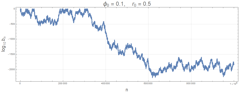
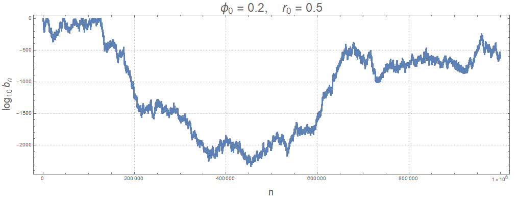
The original recurrence implies for the two new variables $$ b_n ~=~ 1- r_n^2,~~~g_n~=~ \frac{x_n^2}{1-r_n^2}, $$ the recurrence $$ b_{n+1}~=~ 4\,g_n\,b_n^2,~~~ g_{n+1}~=~ \frac1b_n-1-g_n. $$ The question then is whether $b_n\to 0$ for almost all $b_0$ and $$ g_0~=~ \frac{\cos^2 2\,\pi\,t}{b_0}, $$ with equally distributed $b_0,t \in (0,1)$. The original recursion guarantees that $ b_n, g_n>0$. Numerical evaluation runs into the problem of very large exponents, because long sequences easily can lead to $b_n\approx 10^{-1000}$ and $g_n\approx 10^{1000}$. Using these recursions and some home-made C routines to work with very large exponents it is possible to explore the statistics of $b_n$. For any choice of initial conditions $(x_0,y_0)\in D$ one obtains the corresponding $b_0,g_0$ for which the recursion is run for $N=2\times10^6$ steps noting the last iteration step $n=M(x_0,y_0)$ for which $b_n>0.1$. Here are two examples with $N= 10^6$ steps:

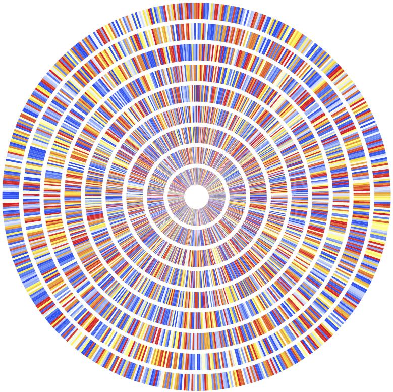
In the plot below each rectangle represent one of these runs for radii $r_0=0.1-0.9$ and angular steps $\Delta\theta_0=0.01$. It shows the spatial distribution of $M(x_0,y_0)/N \in [0,1]$ where red colors are close to 1 and blue colors close to 0 (Mathematica's TemperatureMap). The above two plots correspond to $M/N \approx 0.32$ and $M/N \approx 0.13$. The distribution in the radial plot is not completely random but shows a probably fractal structure, as close values are more likely to be similar.

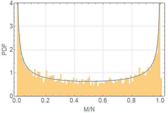
The most interesting observation comes from the statistical distribution of $M(x_0,y_0)/N$ for all runs. Plotted below is the PDF of $M/N$ from the above 5652 runs (yellow) together with the (blue) function $$ f(x) ~=~ \frac{1}{\pi\,\sqrt{x\,(1-x)}}. $$

The data strongly indicate the equality of both distributions, which would imply that $b_n$ almost never converges. The function $f(x)$ is the PDF for the logistic iteration $$ x_{n+1} ~=~ 4 x_n\,(1-x_n),$$ which can be solved by $$x_0 = \sin^2 \frac{\pi}{2}\,t,~~~x_n~=~ \sin^2 \frac{\pi}{2}\,2^n\,t. $$ This solution is very similar to the original iteration for $r_0=1$, but so far I do not see a clear connection for proving that $f(x)$ is the PDF of $M/N$.

Update

From the above definitions one has $$ b_{n+1}~=~ 4\,g_n\,b_n^2~=~4\, x_n^2\,b_n. $$ If $b_n\to 0$, there is $N>0$ such that $r_n>1-\epsilon$ and $b_n<\epsilon$ for $n>N$. One then has $$ b_{N+n}~=~ b_N\,\prod \limits_{k=1}^{n} 4\, x_{N+k}^2 \geq b_N\, \prod \limits_{k=1}^{n} 4\,(1-\epsilon)^{2}\, \sin^2\left( 2^k \theta_N\right). $$ It is therefore of interest to study the behaviour of the products $$ \prod \limits_{k=1}^{n} a\, \sin^2\left( 2^k \theta \right).$$

Because of the logistic iteration above, $f(x)$ is the probability density for the factor $\sin^2\left( 2^k \theta \right)$ in the product $$ \prod \limits_{k=1}^{n} a\, \sin^2\left( 2^k \theta \right).$$ By Birkhoff's ergodic theorem the logarithm of the average factor for $a>0$ is $$\int \limits_0^1 \log(a\,x)\,f(x)\,dx~=~\log\frac{a}{4},$$ such that the average factor is $a/4$. The product $$ \prod \limits_{k=1}^{n} 4\, \sin^2\left( 2^k \theta \right) $$ has average factor 1, but does not converge because $$ 2^k \theta \mod 2\pi $$ is ergodic and thus $ \sin^2\left( 2^k \theta \right)$ does not converge to 1 for almost all $\theta$. Note that the logarithm of the product performs a random walk with step-sizes $$\log 4 + \log \sin^2\left( 2^k \theta \right) $$ where the argument of the last logarithm is distributed according to $f(x)$, such that the step is mostly either very negative or close to $\log 4$.

For constant $a<4$ the product converges to $0$, but in the original iteration one cannot bound $4\,x_n^2$ uniformly away from $4$ and $b_n$ still can diverge (and most likely does).

Update 2

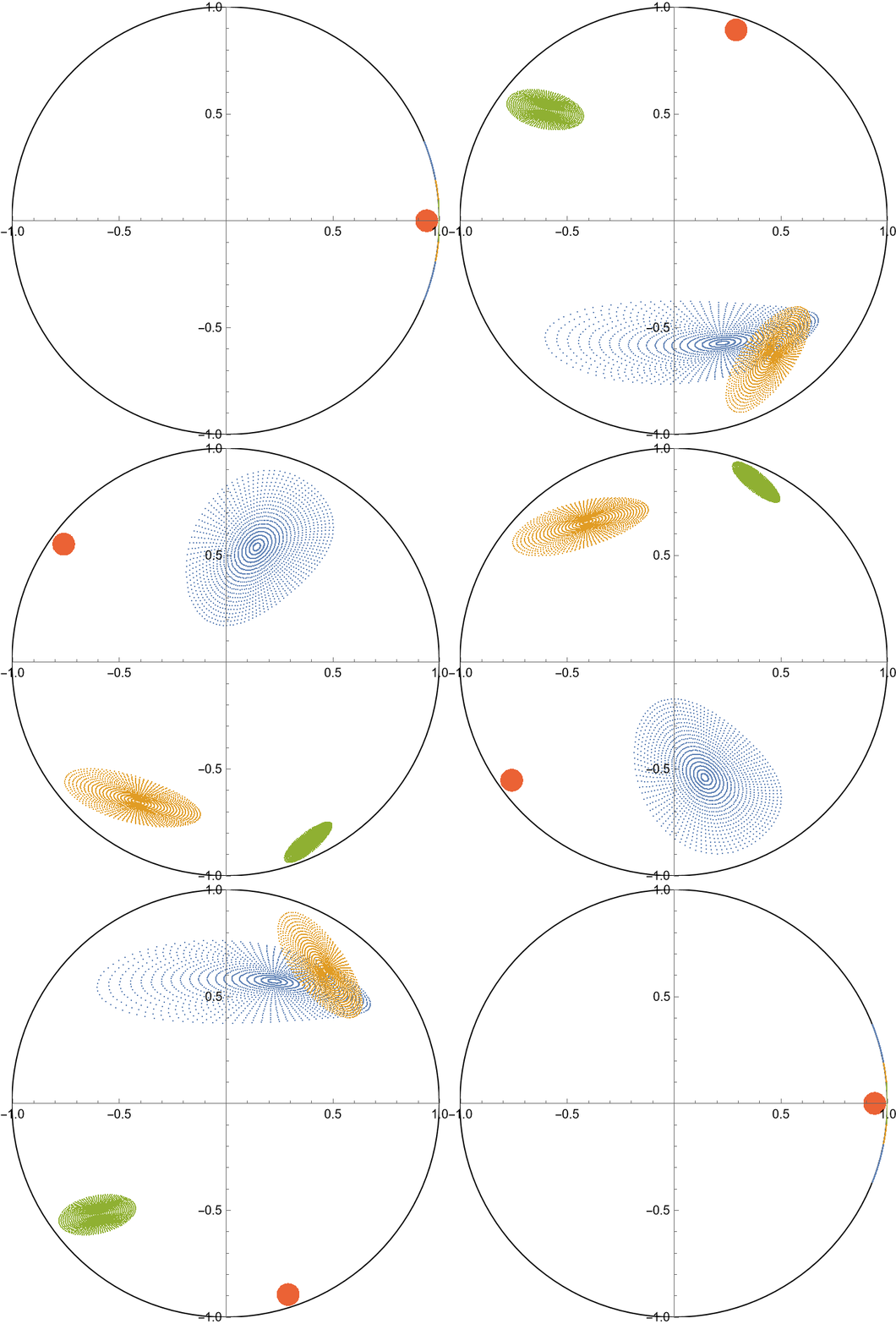
To visualize the topological mapping $T$ considered by @fedja the animation below shows the images $T\,U$ (green), $T^2\,U$ (orange), $T^3\,U$ (blue) of the red disk $U$.

Because exactly the points with $y=0$ map to $(0,1)\in \partial D$ and no other point maps to $ \partial D$, one can iteratively show that exactly the points with $y$ of the form $$ \pm\frac12\,\sqrt{2\pm \sqrt{2\pm \sqrt{2\pm\ldots \sqrt{2 }}}}$$ map to $ \partial D$ after finitely many iterations.

Answer 4

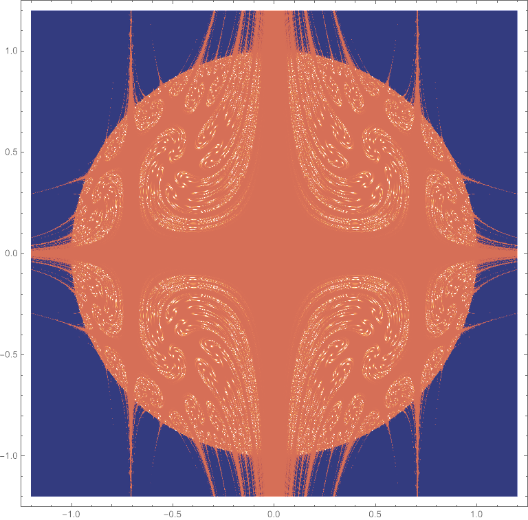
Just another illustration (cw) - color-coded reciprocals of distances from the origin after 14 iterations:

I believe this shows that there is no easy answer...

Answer 5

I still cannot figure out what is going on in the measure-theoretic sense, but the topological dynamics has become a bit clearer. Formally we will show that the set of points that stay sufficiently close to the boundary forever (and, in particular, the set of points that tend to the boundary) is of the first category. I chose to add it as a separate answer because putting three separate messages into one long text will not really facilitate reading. I also fully understand that this observation may be not of research level according to the strict guidelines of MO vigorously imposed by the self-assigned "research police" we have here, but, fortunately, there are no close/delete votes on the answers yet :lol:

So, fix $\varepsilon>0$ to be chosen later. Consider the set $F_m$ of all points that stay within the closed $\varepsilon$-neighborhood of the boundary $D_\varepsilon$ from the $m$-th iteration on. $F_m$ is a closed set, so all we need to show that it has empty interior. Suppose that $U\subset F_m$ is open. Then $T^mU$ is still open and all its images stay $\varepsilon$-close to the boundary. Thus we can start with assuming that $U$ is contained in $D_\varepsilon$ together with all its images. We can also assume that $U$ is small in size.

Now take $z\in U$. Define the argument $A(T^kz)$ of $T^kz$ recursively by choosing some continuous branch of argument in $U$ for $z$ and then making argument of $T^{k+1}z$ close to twice the argument of $T^k z$. Since the argument of $Tw$ is just twice the argument of $w$ up to an additive error of small size $s$ (like $\sqrt\varepsilon$) as long as $w\in D_\varepsilon$, we have no ambiguity in that definition. Moreover, $z\mapsto A(T^kz)$ is continuous in $z$ for fixed $k$ and $|A(T^{k+1}z)-2A(T^kz)|\le s$ for all $k\ge 1, z\in U$.

Now put $a(z)=\lim_{k\to\infty}2^{-k}A(T^k z)$. Since the bounded corrections to the simple doubling dynamics we make are discounted at the exponential rate in that limit (i.e., the correction made at the step $\ell$ contributes only its size times $2^{-\ell}$, the limit exists and is uniform. Thus $a(z)$ is continuous. Moreover, $|A(T^k z)-2^k a(z)|$ is uniformly bounded by the maximal correction size. Those observations have nothing to do with the particular form of $T$. They just apply to any recursion $A_{k+1}=2A_k+s_k$ with $|s_k|\le s$. Then $a=A_1+\sum^j 2^{-j}s_j$ and $A_k=2^k a-\sum_{j>k}2^{k-j}s_j$.

This is the best way I can relate the dynamics inside to that on the boundary. The main issue with doing it in the measure-theoretic way is that I cannot show that $a$ maps a set of positive measure to a set of positive length, so I cannot yet say that the behavior of $T^k e^{ia(z)}$ is generic on the boundary for almost every $z$ inside. However for the topological considerations, we need much less: just that $a(z)$ cannot be constant on $U$.

To show that, assume the contrary. Then the whole neighborhood $U_k=T^kU$ stays within a traveling sector of aperture $2s$ or so $T$ is one-to one on $U_k$. We have the $\mu$-measure of $U_k$ or any subset thereof double every time under our iterations. Now assume that $U_0=U$ had $\mu(U_0)=\nu$ and stayed away from the boundary by $e^{-L}$ (we can always truncate the initial set a bit if it touched the boundary). Then, throwing out the set of the points $z\in U$ where $|2x|<c\frac {\nu}L$ with small $c>0$ (which has $\mu$-measure about $c\nu$), we get after applying $T$ a subset of $TU$ that has $\mu$-measure $2(1-c)\nu>1.5\nu$ and cannot come closer than $e^{-L-C\log(L/\nu)}$ to the boundary. However, the dynamics $(\nu,L)\mapsto (1.5\nu, L+C\log\frac L{\nu})$ eventually makes $\nu$ much greater than $L$, which is impossible because the whole $\mu$-measure of $D_\varepsilon\setminus D_{e^{-L}}$ is about $L$.

Now, once we know that $a(z)$ is not constant, just join two points in $U$ (which we can always assume to be connected) with different values of $a$ by a curve $\gamma_0$ within $U$. Then the image $T_k(\gamma)$ will go around the whole circle a few times and, since anything with $x=0$ is mapped to $(0,1)$ but nothing else is mapped to the boundary, we'll get a closed curve $\gamma$ going around the circle and touching the boundary at $(0,1)$ and $(0,1)$ only in some forward image of $U$.

It remains to show that every such curve contains a point escaping $D_\varepsilon$. To this end, note that $T$ has two continuous in the open disk right inverses $T_+$ and $T_-$ corresponding to the choice of the sign of $x$ in the backward map, i.e., $T_+(x,y)=(\sqrt{\frac {1-y}2}, \frac x{\sqrt{2(1-y)}})$ and $T_(z)=-T_+(z)$. Now choose some point $z_0$ (say, the origin, though it is totally irrelevant) and join it by some curves with $T_-(z_0)$ and $T_+(z_0)$ outside $D_\varepsilon$ (it is here when we need $\varepsilon$ to be not too large in addition to $s$ being not too large). Call the union of these curves $\Gamma$. I claim that one can connect $z_0$ to every its pre-image within the union of all images of $\Gamma$ under all combinations of $T_{\pm}$ is connected.

Indeed, we can connect $z_0$ to $T_{\pm}z_0$ by the construction of $\Gamma$. Suppose that we already know it for the pre-images $T_{\delta_1}\dots T_{\delta_k}(z_0)$. Consider $T_{\delta_1}\dots T_{\delta_{k+1}}(z_0)$. Since $\Gamma$ connects $z_0$ to $T_{\delta_{k+1}}(z_0)$ and the mapping $S=T_{\delta_1}\dots T_{\delta_k}$ is continuous, $S\Gamma$ connects $T_{\delta_1}\dots T_{\delta_{k+1}}(z_0)$ to $T_{\delta_1}\dots T_{\delta_{k}}(z_0)$, but the latter can be connected to $z_0$ by the induction assumption and we are done. Note also that every point in the union of all pre-images of $\Gamma$ ends in $\Gamma$ after some number of iterations and $\Gamma\cap D_\varepsilon=\varnothing$.

However, we have already seen in the Littlewood argument that we have pre-images of $z_0$ with $y\le 0$ that are arbitrarily close to the boundary. In particular, they are outside $\gamma$ while $z_0$ is inside. Thus the union of the pre-images of $\Gamma$ intersects $\gamma$ and we are done.

The topologically chaotic dynamics can usually produce as beautiful pictures as the measure-theoretic chaos. As you can see now, the answer to the topological analog of the OP question is well within our reach, so I don't buy the argument of მამუკა ჯიბლაძე that the (very nice) picture he/she produced indicates that there is no simple answer to the OP's original inquiry. But we'll see :-)

Answer 6

This is not an answer, but I think it provides nice insights.

First reformulation.

Starting from @Karl Fabian reformulation $$ b_{n+1} = 4g_n b_n^2, \ \ g_{n+1} = \frac{1}{b_n} -1 - g_n $$ $$ g_0 = \frac{ \cos^2( 2 \pi t)}{b_0 } $$ with $b_0, t \in (0,1) $ uniformly random, we can substitute $$g_{n+1} = \frac{b_{n+2}}{4 b_{n+1}^2 }, \ \ g_n = \frac{b_{n+1}}{4 b_n^2 } $$ in the second equation and obtain $$ b_{n+2} = \left ( \frac{ b_{n+1} }{ b_n } \right )^2 ( 4 b_n - 4 b_n^2 - b_{n+1} ) $$ If we set $\beta_n = b_{n+1}/b_n$, we get $$ b_{n+2} = \beta_n^2 b_n ( 4 - \beta_n -4 b_n ) $$ Since we'd like to have everything multiplicative, we set $$ \gamma_n = 4 - \beta_n -4 b_n $$ After a few manipulations, we obtain a nice system $$ b_{n+1} = \beta_n b_n $$ $$\beta_{n+1} = \beta_n \gamma_n $$ $$\gamma_{n+1} = (2-\beta_n)^2 $$ With initial conditions $$ \beta_0 = 4 \cos^2(2 \pi t), \ \ \gamma_0 = 4- 4b_0 - 4\cos^2(2 \pi t) $$ As a sanity check, you can verify that the identity $4b+\gamma+\beta=4$ is preserved when applying the recurrence. Since we have a lot of multiplications involved, we'd like to take logarithms. As long as we start with positive initial conditions, we can consider $X_n = \log(b_n), Y_n = \log(\beta_n), Z_n = \log(\gamma_n)$ and we reduce to $$ X_{n+1} = X_n + Y_n $$ $$ Y_{n+1} = Z_n+ Y_n $$ $$ Z_{n+1} = f(Y_n) $$ where $f(s) = 2 \log | 2- e^s | $.

First experiment. I have implemented the program and tried random starting values. There is a small trick to do in order to deal with very negative values of $X$, to prevent approximations to make the system explode (namely, I force the y-variable to preserve the $\alpha-\beta-\gamma$ linear condition hold at each step, which has to be the case algebraically).

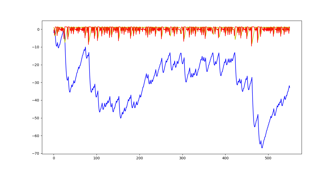
This is a plot with 1000 iterations, where $X$ is blue, $Y$ is red, $Z$ is yellow. Recall that $X= \log b$ is the logarithm of the radius, the variable we are interested in: It seems to go to $-\infty$ also when we add more iterations.

Second reformulation. The above system furnishes a way to reduce to a nice, single variable recurrence. If we substitute $Z_{n+1} = Y_{n+2} - Y_{n+1}$ in the last equation, we get $$ Y_{n+2} = Y_{n+1} + f(Y_n)$$ The variable we are interested in is the associated series: $$ X_{n+1} = \sum_{k=0}^n Y_k $$ The only nice thing I have managed to show is the following: $Y$ change sign infinitely many times.

Part 1: $Y_n \le \log(3)$.

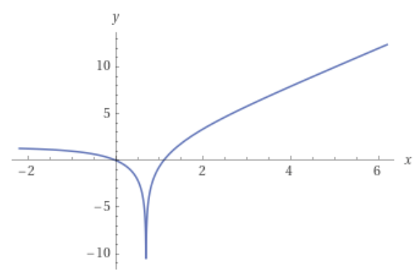
Since $\gamma = (2-\beta)^2 \ge 0$ and $b = 1-r^2 \ge 0$ because the original recurrence preserves the unit disk, we have that $$ Y = \log \beta = \log ( 4- 4b - \gamma) \le \log(4) $$ So that $Y$ is bounded. Note that the function $f$ has the following plot:

with zeroes at $0, \log(3)$. We want to show that it is impossible to have $Y_n, Y_{n+1} > \log(3)$. Indeed, in this case: $$ Y_{n+k+2} = Y_{n+k+1} + f(Y_{n+k}) > Y_{n+k+1} + \varepsilon $$ since $f$ is increasing and positive above $\log(3)$. This contradicts the boundedness of $Y$.

On the other hand, let us also notice that there is no uniform (with respect to initial conditions) bound from below to $Y$: since there is a 'pitfall' around $\log(2)$, that is $\lim_{s \to \log(2) }f(s) = -\infty$, if $Y_n \approx \log(2)$ we will have $Y_{n+2} = Y_{n+1} + Y_n $ negative and very large in absolute value.

Part 2: oscillation.

Suppose $Y_n, Y_{n+1} < 0$ for some $n$. Let $\varepsilon$ small enough so that $Y_n, Y_{n+1} < \log(1-\varepsilon) $. It is easy to see that, since $f$ is decreasing below zero, $f(t) \ge f(\log(1-\varepsilon)) = 2 \log(1+\varepsilon) $ for $t \le \log(1-\varepsilon) $. Suppose that $Y_{n+k} \le \log(1-\varepsilon)$ for all $k \ge 0$. Then: $$ Y_{n+k+2} = Y_{n+k+1} + f(Y_{n+k}) \ge Y_{n+k+1} + 2 \log(1+\varepsilon) $$ which implies $\lim_{k \to \infty} Y_{n+k} = \infty$, in contradiction with the assumed boundedness. Thus we have $Y_{n+k} > \log(1-\varepsilon)$ for the first time at some $k$. At the next iteration, we will have $$ Y_{n+k+1} \ge Y_{n+k} + 2\log(1+\varepsilon) > \log(1-\varepsilon) + 2\log(1+\varepsilon) \approx \varepsilon > 0 $$ For $\varepsilon$ small enough. The other direction is analogous, with a little variation due to the fact that $f$ is less nice for positive arguments. We can still argue that $f(Y) \le 2\log(1-\varepsilon)$ as long as $Y \ge \log(1+\varepsilon)$ and $\varepsilon$ is small enough. Firstly, since $Y_n < \log(3)$, the sequence will decrease as long as $Y$ stays positive. Secondly, in the interval $( \log(1+\varepsilon), Y_n )$ the function has maximum given by $ 2 \log(1-\varepsilon)$.

Last observation. It seems like a 'fractal' behavior could be possible, in the following weak sense. Let $D$ be the unit disk and fix some large $L << 0$. Let $\ell : D \to \mathbb{N}$ be defined so that $\ell(z)$ is the minimum value for which $X_n \le L$ whenever $n \ge \ell(z)$.

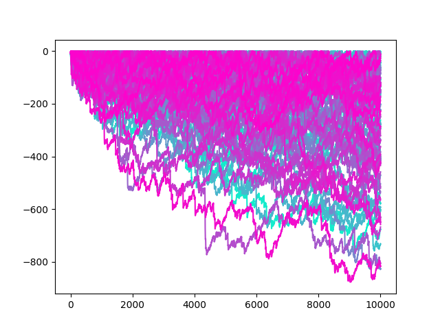
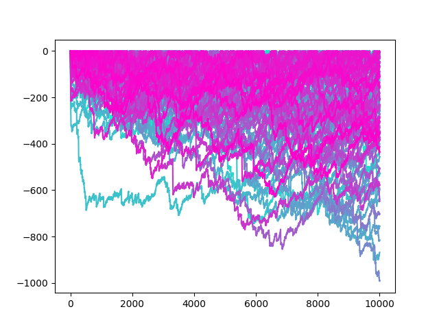
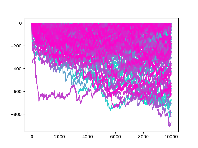
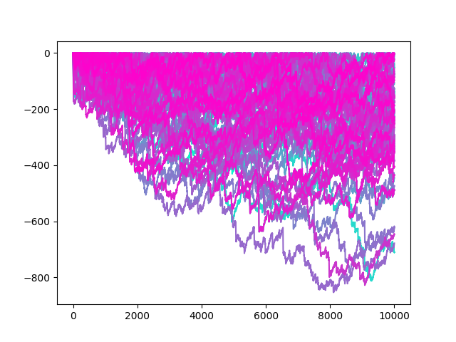
There could exist a function $F: D \to D$ such that $\ell(F(z)) \ge C \ell(z)$ with $C > 1$ a constant. In this way $M_k:= F^{(k)}(D)$ has bigger and bigger convergence times as $k$ increases, and $M_{\infty} := \bigcap_{k \ge 0} M_k $ is an interesting fractal with unknown behavior (but possibly non-converging). This conjecture is partly supported by the following plot observations: plotting many starting values at different scales (100 samples, p1: t=0.01-0.02, p2 t=0.1-0.2,p3: t=0.3-0.4, p4:t= 0.01-0.049), there seems to be a strikingly similar behavior:

In the 'pitfall' perspective, I think one of the main questions is whether or not we can hit a neighborhood of the pitfall infinitely many times. Intuitively, once we get a very negative $Y$ value $-L$, we will go upward of $\approx 2 \log(2 - e^{-\infty}) = 2 \log(2) \approx 1.386 $ at each step. If $L/ \log(2)$ is odd, at the last step we will land around $\log(2)$, yielding another big step (neglecting the fact that the approximation fails to hold in the last steps...); if it is even, we will likely end close to zero, and numerical experiments suggest it will keep oscillating around zero. It would be nice to:

1. Find a threshold $\alpha$ such that $|Y| \le \alpha$ is an invariant subset;
2. Estimate the sum of $Y$ terms in a 'pitfall cycle', when $Y$ goes close to $\log(2)$ and then becomes very negative, until it gets positive again;
3. Estimate the sum of $Y$ terms in a 'oscillation cycle', when $Y$ is within the threshold $\alpha$.

Note that $\alpha$ small enough does not work, since $Y$ escapes the small regime. Indeed, as long as $Y$ is small, since $f(s) \approx - 2s$ for $s$ small, we have that $$ Y_{n+2} = Y_{n+1} + f(Y_n) \approx Y_{n+1} - 2Y_n $$ The latter has characteristic roots $\lambda, \bar{\lambda}$ where $\lambda = 2 e^{i \theta}$ and $\theta \approx 0.42 \pi$. This system evolves as $$ Y_n = \alpha \lambda^n + \bar{\alpha} \bar{\lambda}^n = \textrm{Re}(\alpha \lambda^n) = \rho 2^n \cos( n \theta + \phi) $$ for some $\alpha = \rho e^{i \phi} $. This proves the sequence gets bigger and bigger until the approximation regime is no longer valid.