1
$\begingroup$

I hope this is an appropriate forum for this question, and I asked on math.stackexchange as well. If it doesn't belong, I don't mind closing this. If my questions is not clear, please just let me know and I'll try to add information/explanation where I can.

Say I have a set of data points that I run through a FLAME clustering algorithm, and I get my set of cluster supporting objects, and the fuzzy memberships among them.

Next, let's say I get an additional set of data, for argument's sake, let's say it doubles the amount of data. If I want to add that to my clustering, without having to reprocess the old data (i.e. just using the cluster supporting objects, and adding these new observations to the cluster), will I be introducing some kind of bias? To get the most "accurate" picture, would it be better to reprocess ALL the data, re-establish CSO's, re-compute distances, etc.?

To add to the complexity, let's say I'm going to be periodically adding similar quantities of data points. Does the answer to the above change?

And I guess a final question - is there a clustering algorithm (or family of algorithms) that is not subject to extreme bias in the beginning, such that added data points can be added relatively pain-free? I'm sort of thinking that FLAME clustering, with its nice fuzziness properties is a reasonable way of going about this, but any more suggestions would be helpful.

Thanks!

$\endgroup$

3 Answers 3

1
$\begingroup$

It is intrinsic to the finite sampling of a dataset to have a "variance" that affect clustering results, and this is not a matter of the algorithm.

Algos have parameters, like the K number of neighbors in FLAME, that adjust for this variance but, on the other side, introduce a "bias".

Thus what happens usually is that you choose a K that is large enough to be robust to your sample, but not too large for estimating an "informative" model. (Obviously you cannot do better than noise) (see for example:http://www.math.princeton.edu/~amits/publications/laplacian_ACHA.pdf)

An interesting criterion to use is that of stability: if samples with the same cardinality of your data give similar clustering results then you can, heuristically, avoid recomputations. On the other hand, if your data are too few you should recompute your model each time new data arrives.(or wait you have enough data) (link:http://arxiv.org/abs/1007.1075)

$\endgroup$
1
$\begingroup$

I've looked at this for PCA-based clustering.

alt text

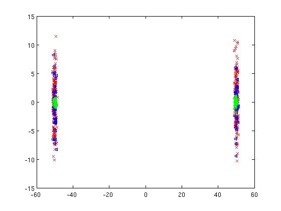
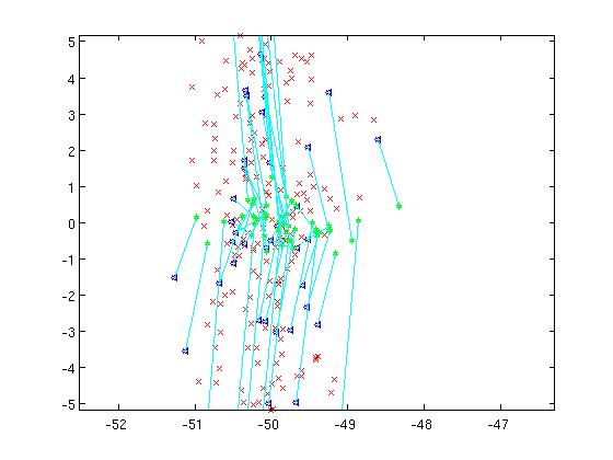
Here is some PC clustering of a simulated dataset. We first draw the clusters as red xs on PCs computed from the entire dataset. A few random points (these are marked blue) are removed from the dataset and the PCs are computed on reduced data. The blue data are then plotted against the reduced PCs and colored green.

alt text

I don't have a rigorous bound (I would really like some references) but from what I can tell the most drastic changes are in directions that involve only noise.

Here is some matlab code:

clear all;close all;clc;

%create garbage SNP-style data
m = 500;
n = 25000;
M = zeros(m,n);

%create 2 populations
%one has 0s in the interesting columns
%the other has 2s
interesting_variables = randsample(1:n, .1*n);
M(1:2:m, interesting_variables) = 2.0;

%add sampling noise
sigma = 4.0;
M = M + double(sigma*randn(m,n) > ones(m,n));

%center data
for j=1:n
    M(:,j) = M(:,j) - mean(M(:,j));
end

% plot PCA based clusters, Tygert's code is faster.
tic
[~,~,V] = svds(M,2);
toc


coordsx = zeros(1,m);
coordsy = zeros(1,m);
for i=1:m
    coordsx(i) = M(i,:)*V(:,1);
    coordsy(i) = M(i,:)*V(:,2);
end

figure()
title('strcuture')
plot(coordsx, coordsy, 'rx')


%% 
% Now pick some guys from the dataset to monitor
% identify them as blue triangles in the plot
%

some = m/5;
guys = randsample(1:m, some);

hold on;
coordsx_blue = zeros(1,some);
coordsy_blue = zeros(1,some);
for i=1:some
     coordsx_blue(i) = M(guys(i),:)*V(:,1);
     coordsy_blue(i) = M(guys(i),:)*V(:,2);
end
plot(coordsx_blue, coordsy_blue, 'b<');


%%
% Finally, run PCA again but without the blue guys.
% Observe how this changes the clustering when we plot the blue
% against the PCs found from the reduced data
% green is the new blue.
%

M_small = M;
M_small(guys, :) = [];
[ms ns] = size(M_small);

tic
[~,~,V_small] = svds(M_small,2);
toc

coordsx_newblue = zeros(1,some);
coordsy_newblue = zeros(1,some);
for i=1:some
    coordsx_newblue(i) = M(guys(i),:)*V_small(:,1);
    coordsy_newblue(i) = M(guys(i),:)*V_small(:,2);
end
plot(coordsx_newblue, coordsy_newblue, 'gh');


% draw some lines to see how things moved
for i=1:some
    line([coordsx_blue(i) coordsx_newblue(i)], [coordsy_blue(i) coordsy_newblue(i)],'Color','c');
end
$\endgroup$
0
$\begingroup$

Can you give a few more specifics about the problem? What is the dimensionality of the data; what are representative data set sizes? Perhaps a little more about the motivation of the underlying problem?

$\endgroup$

You must log in to answer this question.

Not the answer you're looking for? Browse other questions tagged .