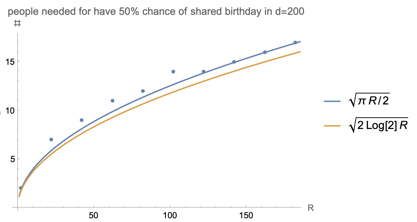
$\newcommand{\PP}{\mathcal P}\newcommand{\np}{\|\mathbf p\|}\newcommand{\pmax}{p_{\max}}\newcommand{\X}[2]{X_{\{#1,#2\}}}\newcommand{\sub}[3]{#1_{\{#2,#3\}}}\newcommand{\Ga}{\Gamma}\newcommand\la\lambda$The correct constant factor is, not $\sqrt{\pi/2}=1.253\ldots$, but
\begin{equation*}
c_*:=\sqrt{2\ln2}=1.177\ldots. \tag{10}\label{10}
\end{equation*}
Indeed, let $Y_1,\dots,Y_d$ be independent random variables (r.v.'s) such that $P(Y_a=j)=p_j$ for all $a\in[k]:=\{1,\dots,k\}$ and $j\in[d]$. Let $\PP_k$ denote the set of all subsets of $[k]$ of cardinality $2$. For each set $\{a,b\}\in\PP_k$, let
\begin{equation*}
\X ab:=1(Y_a=Y_b).
\end{equation*}
Let
\begin{equation*}
\np:=\sqrt{\sum_{j\in[d]}p_j^2}\quad\text{and}\quad \pmax:=\max_{j\in[d]}p_j.
\end{equation*}
Let
\begin{equation*}
P_k:=P(S_k=0),\quad\text{where}\quad S_k:=\sum_{\{a,b\}\in\PP_k}\X ab. \tag{20}\label{20}
\end{equation*}
Theorem 1. If
\begin{equation*}
\np\to0, \tag{25}\label{25}
\end{equation*}
\begin{equation*}
\pmax=o(\np), \tag{30}\label{30}
\end{equation*}
and
\begin{equation*}
k\sim\frac c\np \tag{40}\label{40}
\end{equation*}
for some real $c>0$, then
\begin{equation*}
P_k\to e^{-c^2/2}. \tag{50}\label{50}
\end{equation*}
In particular, if $c=c_*$ (with $c_*$ as in \eqref{10}), then
\begin{equation*}
P_k\to1/2.
\end{equation*}
Remark: Condition \eqref{30} means that the effective number, $\np^2/\pmax^2$, of "calendar dates" in this non-uniform version of the birthday "paradox" is large. In particular, if $p_1=\cdots=p_d=1/d$, then this effective number of "calendar dates" is $d$, the actual number of "calendar dates" in the usual, uniform version of the birthday "paradox".
Remark: The probability $P_k$ can be interpreted as the probability of not having the same birthday for any two of the $k$ i.i.d. individuals given that, for each $j\in[d]$, the probability of a birthday on day $j$ is $p_j$.
The proof of Theorem 1 is a direct application of a result on Stein's method for Poisson approximation. Such an application is possible because the random indicators $\X ab$ are almost independent.
Specifically, in Theorem 2.5 on p.70, let $\Ga:=\PP_k$,
$\sub\Ga ab^s:=\{\{c,d\}\in\Ga\colon|\{c,d\}\cap\{a,b\}|=1\}$, and
$\sub\Ga ab^w:=\{\{c,d\}\in\Ga\colon|\{c,d\}\cap\{a,b\}|=0\}$, where $|\cdot|$ denotes the cardinality.
Note that for each $i\in\Ga$ we have $EX_i=\np^2=E(X_i|W_i)$ (since $X_i$ is independent of $W_i=\sum_{j\in\Ga_i^w}X_j$) and hence
\begin{equation*}
\la=\binom k2\np^2\sim k^2\np^2/2\to c^2/2; \tag{60}\label{60}
\end{equation*}
$EZ_i\le2k\np^2$; and $EX_iZ_i\le2k\np^2\pmax$. Also, $k_2(\la)\le1$ (and also $k_1(\la)\le1$, but in this case $k_1(\la)$ will get multiplied by $0$ anyway). We thus conclude that
\begin{equation*}
|P_k-e^{-\la}|\le\frac{k^2}2\,(\np^2(\np^2+2k\np^2)+2k\np^2\pmax)\to0,
\end{equation*}
in view of the conditions \eqref{25}, \eqref{30}, and \eqref{40}. So, in view of \eqref{60}, we get \eqref{50}. $\quad\Box$
Relation \eqref{50} is illustrated in this Mathematica notebook. At the end of the notebook, one can see graphs $\{(c,\tilde P_k/e^{-c^2/2})\colon c\in\frac{c_*}5\,\{1,\dots,10\}\}$ for simulated values $\tilde P_k$ of $P_k$, $p_j=j/\sum_{i\in[d]}i$ for $j\in d$, $k=\lceil c/\np\rceil$, $d=500$ with $1000$ simulations (penultimate graph), and $d=1000$ with $2000$ simulations (last graph). We see good agreement with \eqref{50} for values of $c$ around and/or to the left of $c_*$, but this agreement seems worse for larger values of $c$ -- which may be caused by relatively small values of the limit probability $e^{-c^2/2}$, which is therefore harder to simulate.
Added: A result more general than Theorem 1 above is Theorem 4 by Camarri and Pitman, which states the following (in terms of the present answer):
Suppose that $\pmax\to0$ (which of course implies $d\to\infty$ and is equivalent to \eqref{25}).
Suppose also that
for each $j=1,2,\dots$ and some $t_j$ we have
\begin{equation}
p_j/\np\to t_j. \tag{70}\label{70}
\end{equation}
(So, necessarily $t_j\in[0,1]$ for all $j$.) Then, for $k$ as in \eqref{40},
\begin{equation*}
P_k\to Q(c):=e^{-c^2(1-\sum_j t_j^2)/2}\prod_j(1+t_j c)e^{-t_j c}. \tag{80}\label{80}
\end{equation*}
Moreover, condition \eqref{70} is necessary for $P_k$ to converge for all real $c>0$.
(Thanks to kodlu for the link to a question containing a reference to the paper by Camarri and Pitman.)
Clearly, Theorem 1 in this answer is a special case of the just stated theorem by Camarri and Pitman: specifically, our Theorem 1 corresponds to the case when $t_j=0$ for all $j$. However, the proof of Theorem 1 presented above seems much simpler than the proof of the theorem by Camarri and Pitman. Also, the equation $e^{-c^2/2}=1/2$ is much easier to solve (to get the solution $c=c_*$ as in \eqref{10}) than the equation $Q(c)=1/2$ in general, with $Q(c)$ as defined in \eqref{80}.

