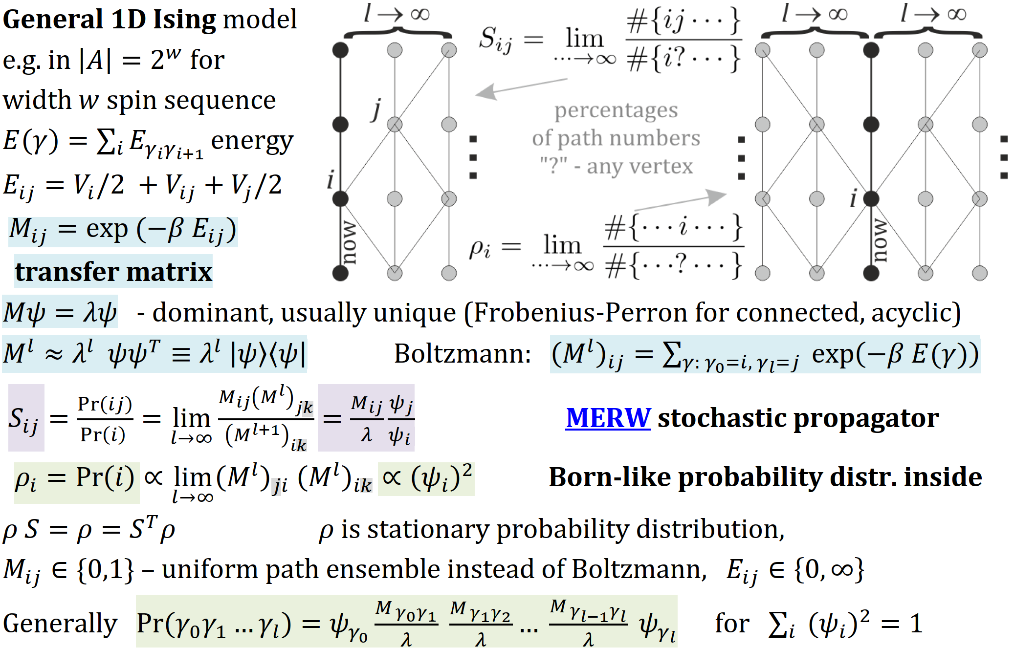
I was reading the paper 0810.4113v2, burda, which analyzed the stationary distribution maximal entropy random walk on the irregular lattice. I am confused on some of the steps.
Description:
The graph is defined by asymmetric adjacency matrix $A$, with elements $A_{ij} = 1$ if $i$ and $j$ are neighboring nodes and $A_{ij} = 0$ otherwise. The hopping is a local Markov process: the particle which arrives at some moment to node $i$ will hop to a neighboring node $j$ with probability $P_{ij}$, independently of the past history. The elements of the transition matrix are $P_{ij} = 0$ if $A_{ij} = 0$, that is if nodes $i$, $j$ are not linked, and for each $i$ one has $\sum_j P_{ij} = 1$.
The main quantity of interest is the probability, $\pi_i(t)$, of finding the particle at node $i$ at time $t$. One can calculate it recursively, applying the Markov property: $$\pi_i(t + 1) = \sum_j\pi_j(t)P_{ji}. ~~~~~~~~(1)$$
Using spectral properties of the matrix $P_{ij}$ , one can show that πi(t) reaches for $t \rightarrow \infty$ a unique stationary state $\pi^*_i$ obeying the following eigenequation: $$\pi^*_i=\sum_j\pi^*_j P_{ji}. ~~~~~~~~(2)$$
........
Let $\psi_i$ be the normalized eigenvector, $\sum_i \psi^2_i=1$, corresponding to the maximal eigenvalue $\lambda$ of the adjacency matrix $A_{ij}$: $$\sum_j A_{ij}\psi_j = \lambda\psi_i.~~~~~~~~(6)$$
The eigenvalue $\lambda$ is clearly in the range $k_{min} \leq \lambda \leq k_{max}$ ,where $k_{min}$ and $k_{max}$ are the maximal and minimal node degrees of the graph, respectively. The Frobenius-Perron theorem tells us that the eigenvetor has all elements of the same sign, so that one can choose $\psi_i > 0$. Let us use this eigenvector to define the following transition matrix: $$P_{ij}=\frac{A_{ij}}{\lambda}\frac{\psi_j}{\psi_i}.~~~~~~~~(7)$$
By construction, the entries $P_{ij}$ are positive if $i$ and $j$ are neighboring nodes. They are also properly normalized:$\sum_j P_{ij} = 1$. A similar onstrution has been reently proposed in the ontext of optimal information coding [7]. The weight (4) is now independent of intermediate nodes: $$P(\gamma^{(t)}_{i_0~i_t}) = \frac{1}{\lambda^t}\frac{\psi_{i_t}}{\psi_{i_0}},~~~~~~~~(8)$$ and thus all trajectories having length $t$ and given endpoints $i_0$ and $i_t$ are equiprobable. For a closed trajectory, the probability (8) depends only on its length $t$. The stationary distribution of MERW is $$\pi^*_i=\psi^2_i~~~~~~~~(9)$$ which is easy to check by combining Eqs. (7) and (2). It is a normalized probability: $\sum_i\pi^*_i=1$, and the detailed balance condition is fulilled: $\pi^*_i P_{ij}=\pi^*_j P_{ji}$.
I am confused about how to obtain (9). Does any one can give me the detail intermediate steps to obtain (9)? Thanks in advance.
I tried:
$$\pi^*_i=\sum_j\pi^*_jP_{ji}$$ $$j\rightarrow i, P_{ji}=\frac{A_{ji}}{\lambda}\frac{\psi_i}{\psi_j}$$ $$i\rightarrow j, P_{ij}=\frac{A_{ij}}{\lambda}\frac{\psi_j}{\psi_i}$$ $$\pi^*_i=\sum_j\pi^*_jP_{ji}$$ $$=\sum_j(\sum_i\pi^*_i P_{ij})P_{ji}$$ $$=\sum_j\sum_i\pi^*_i P_{ij}P_{ji}$$ $$=\sum_j\sum_i\pi^*_i \frac{A_{ij}}{\lambda}\frac{\psi_j}{\psi_i}\frac{A_{ji}}{\lambda}\frac{\psi_i}{\psi_j}$$ $$????~~~~=\psi^2_i~~~~????$$
I also read ref Maximal_entropy_random_walk. I still confused.

