Optimization of a continuous function

Question

This is more like an optimization problem but any solution is appreciated.

I have a data set with input specifying power(demand) to be generated for a particular time period(TP).

Input:
Time --- Power
01 to 02 1000
02 to 03 2000
03 to 04 2000
04 to 05 1500
etc.,

But the power can't just be increased from 1000 to 2000 at 01:59:59. Here there will be some ramping rate(gradient) which I want to minimise by keeping the imbalance to 0. Imbalance may arise if you deviate from what is needed, here power cannot be more or less than what is required in that Time Period.

In summary I have to generate the black line(which is output) below (red line is the input).

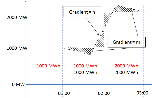
I am trying to get an output which can be a curve(black line) equation or the power to generate at the deflection points(say at around 1:45 we generate 800 then at 2:15 it can be 2200 which will keep the imbalance to 0).

When I tried to treat this as an optimization problem it may look something like this:
Objective : Minimise gradient f(x) = Yj-Yi/Xj-Xi between 2 points (Xi,Yi) and (Xj,Yj)
Subject to constraints:

average of Yi = Power value(redline in that Time Period)

But I am struggling to complete it how to represent mathematically to be able to implement using programming like R's lpsolve/optimize or Python's scipy optimizers.

Any help on the approach to take would be greatly appreciated.

Answer 1

Here is just a recipe. It has its advantages and disadvantages, so try to implement it and see if it gives what you want or there are some undesirable features. It minimizes the integral of the gradient squared on a long run while preserving the average over each interval $[k,k+1]$ where $k$ is an integer.

1) Compute the coefficients $a_k=\frac 1{2\pi}\int_0^{2\pi}\frac{3\cos kt\,dt}{2+\cos t}$, $k=0,1,2,\dots$. About $10$ of them should be enough for decent precision.

2) Define $f(x)$ to be $0$ if $x\le-1$; $(x+1)^2/2$ if $-1\le x\le 0$, $1-(1-x)^2/2$ if $0\le x\le 1$, $1$ if $x\ge 1$.

3) Define the "elementary response" $$ g(x)=a_0 f(x)+\sum_{k\ge 1} a_k[f(x-k)+f(x+k)]\,. $$

4) If your time interval is $[0,T]$, then your curve is $$ Y(x)=\text{Average}_{[0,1]}Y+\sum_{t=1}^{T-1} \Delta Y(t) g(x-t) $$ where $\Delta Y(t)$ is the difference of the averages over $[t,t+1]$ and $[t-1,t]$ (so the elementary response corresponds to the output that is $0$ for negative times and $1$ for positive times).

Test it and let me know if you have any problems with this solution.