added 170 characters in body
Source Link

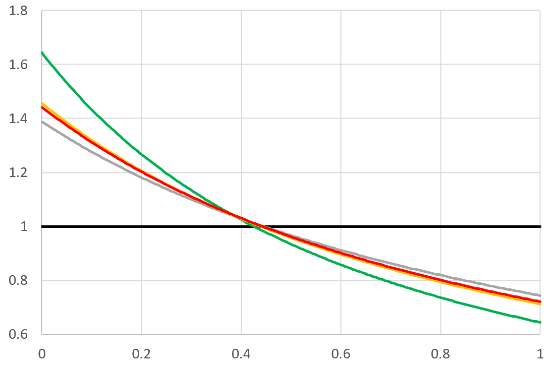
In practice, using the first few hundreds terms in the infinite sum, and using a few thousand values of $x$ evenly spread in $[0, 1]$, provides a good approximation to $f_X(x)$ within only $3$ or $4$ iterations. In the cases tested, convergence occurred when $\lambda\leq 1$. The chart below shows the first $4$ iterations with $\lambda=\alpha=1$. In that case, the theoretical $f_X$ is known and represented by the red curve in the figure below. The black line is the initial uniform density $f_0$ on $[0, 1]$. The green curve corresponds to $f_1$, the grey one to $f_2$, and the orange one to $f_3$. The orange one is very close to $f_X=f_\infty$: one can barely distinguish it from the red curve.

A Perl script for the fixed point iterations is available here. Note that there are infinitely many solutions to the functional equation (multiples of each other), but there is only one that is a density, that is, integrating to $1$.

In practice, using the first few hundreds terms in the infinite sum, and using a few thousand values of $x$ evenly spread in $[0, 1]$, provides a good approximation to $f_X(x)$ with only $3$ or $4$ iterations. In the cases tested, convergence occurred when $\lambda\leq 1$. The chart below shows the first $4$ iterations with $\lambda=\alpha=1$. In that case, the theoretical $f_X$ is known and represented by the red curve in the figure below. The black line is the initial uniform density $f_0$ on $[0, 1]$. The green curve corresponds to $f_1$, the grey one to $f_2$, and the orange one to $f_3$. The orange one is very close to $f_X=f_\infty$: one can barely distinguish it from the red curve.

A Perl script for the fixed point iterations is available here.

In practice, using the first few hundreds terms in the infinite sum, and using a few thousand values of $x$ evenly spread in $[0, 1]$, provides a good approximation to $f_X(x)$ in only $3$ or $4$ iterations. In the cases tested, convergence occurred when $\lambda\leq 1$. The chart below shows the first $4$ iterations with $\lambda=\alpha=1$. In that case, the theoretical $f_X$ is known and represented by the red curve in the figure below. The black line is the initial uniform density $f_0$ on $[0, 1]$. The green curve corresponds to $f_1$, the grey one to $f_2$, and the orange one to $f_3$. The orange one is very close to $f_X=f_\infty$: one can barely distinguish it from the red curve.

A Perl script for the fixed point iterations is available here. Note that there are infinitely many solutions to the functional equation (multiples of each other), but there is only one that is a density, that is, integrating to $1$.

Added the section "solving the functional equation"
Source Link

Solving the functional equation

We can use the above formula to implement a fixed point algorithm that converges to the density $f_X$, starting with $n=0$ and a uniform density $f_0$ on $[0, 1]$, and using the following recursion:

$$f_{n+1}(x)=\sum_{k=1}^\infty |g'(x)|\cdot f_n(g_k(x), \mbox{ } \mbox{ } \mbox{ } 0\leq x \leq 1. $$

In practice, using the first few hundreds terms in the infinite sum, and using a few thousand values of $x$ evenly spread in $[0, 1]$, provides a good approximation to $f_X(x)$ with only $3$ or $4$ iterations. In the cases tested, convergence occurred when $\lambda\leq 1$. The chart below shows the first $4$ iterations with $\lambda=\alpha=1$. In that case, the theoretical $f_X$ is known and represented by the red curve in the figure below. The black line is the initial uniform density $f_0$ on $[0, 1]$. The green curve corresponds to $f_1$, the grey one to $f_2$, and the orange one to $f_3$. The orange one is very close to $f_X=f_\infty$: one can barely distinguish it from the red curve.

enter image description here

A Perl script for the fixed point iterations is available here.

Source Link

My answer applies to standard continued fractions $x_0=[a_0,a_1,\dots]$ corresponding to $\alpha=1$, as well as to the full general case. As stated in my original question, the $a_n$'s are called the digits of $x_0$ in the continued fraction system (actually, continued power if $\alpha\neq 1$). The following is true for all normal numbers $x_0$ in that system, with the definition of normality being a generalization of the concept as we know it in base $10$ or base $2$. All numbers $x_0\in[0,1]$ but a set of Lebesgue measure zero, are normal in the continued power numeration system. Yet the set of non-normal numbers is dense.

That said, let's now answer my question. The theoretical distribution $D$ of any digit $a_n$ of any normal number $x_0$ in the power system, satisfies the following:

  1. It is unbounded, that is, $P(D=k)>0$ for any strictly positive integer $k$
  2. $P(D=k) \sim O(k^{-(1+1/\alpha)})$ as $k\rightarrow\infty$
  3. $E(D)$ is infinite if and only if $\alpha\geq 1$
  4. $Var(D)$ is infinite if and only if $\alpha\geq \frac{1}{2}$

The correlation between successive digits thus exists if $\alpha<\frac{1}{2}$.

Proof of the main result (sketch)

Let $X$ be the random variable associated with the equilibrium distribution of the sequence $(x_n)$. We have

$$P(D=k)=P(m_{k+1}<X\leq m_k)=\int_{m_{k+1}}^{m_k} f_X(x)dx \sim O(m_k-m_{k+1})$$

where $m_k=(\lambda/k)^{1/\alpha}$. Since $f_X(x)$ is bounded, smooth, and away from zero in $[0,1]$, results 1 and 2 follow easily. The asymptotic result is based on the fact that $f_X$ is quite close to a uniform density on $[0,1]$.

We also have

$$E(D)=\int_0^1 \frac{\lambda}{x^\alpha}f_X(x)dx - \int_0^1 \Big\{\frac{\lambda}{x^\alpha}\Big\}f_X(x)dx$$ where the curly brackets represent the fractional part function. The rightmost integral is finite, and the left one is infinite only if $\alpha\geq 1$. Now we proved the third result. A similar argument can be used to prove the last result. Note that for continued fractions ($\alpha=\lambda=1$) the distribution of $D$ is known exactly, and verifies all the properties 1-4 listed above.

Functional equation for $f_X$

Let $x'$ be a back image of $x$, in the sense that if $x_{n+1}=x$, then $x_{n}=x'$. For any $x\in [0,1]$, there are infinitely many back images $x_k'$ indexed by $k=1,2,\dots$ and denoted as

$$x_k'=g_k(x) = \Big(\frac{\lambda}{x+k}\Big)^{1/\alpha}.$$

Now the back image of the whole interval $[x,x+\epsilon]$ (with $\epsilon$ very close to $0$) is $$\bigcup_{k=1}^\infty \Big[g_k(x+\epsilon),g_k(x)\Big].$$ The length of the $k$-th interval in the above formula is approximately $\epsilon g'_k(x)$, where $g'$ denotes the derivative with respect to $x$. Thus, we have the following fundamental functional equation: $$f_X(x)=\sum_{k=1}^\infty |g'_k(x)|\cdot f_X(g_k(x)) .$$

In particular, if $\alpha=\lambda=1$ (the standard continued fraction), it is easy to verify that $f_X(x)=\frac{1+x}{\log 2}$ satisfies the above formula and is thus the density associated with the equilibrium distribution. This is a well known result, and the proof provided here is probably one of the shortest ones.