added 3178 characters in body
Source Link

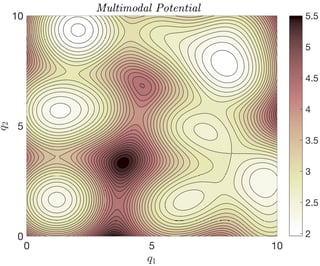
Let me elaborate a bit on the parallel tempering method and what makes it a surprising example. The aim of the method is to sample from a probability distribution with a multi-modal energy landscape, which one can regard as a high-dimensional version of:

enter image description here

The difficulty with sampling from a probability distribution with an energy landscape like this one is not only the fact that there are many modes, but that the energy barriers between these modes may be too high for a simple MCMC method to overcome. Simply put, even computing the mean and variance of this distribution might be impractical to do using simple MCMC methods.

The basic idea in parallel tempering is to introduce a fictitious temperature parameter that flattens the desired probability distribution, and hence, makes it easier to sample from using a simple MCMC method. Then one constructs a sequence of distributions from a sufficiently flat distribution (at high temperature) to the desired probability distribution (at lower temperature). Then one runs a sequence of chains to sample from this sequence of distributions.

Each of these chains evolves at its own temperature, but occasionally one swaps the states between these chains so that the chain running at the lowest temperature explores its landscape more efficiently. (Unfortunately the samples generated at the higher temperatures cannot be directly used to sample from the desired distribution at the lowest temperature in the sequence.)

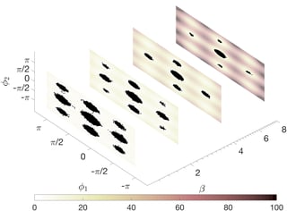
As a concrete example, consider applying parallel tempering to a 15 degree of freedom pentane molecule. The goal here is to sample from the equilibrium distribution of this molecule in the plane defined by its two dihedral angles (these are certain internal degrees of freedom of the molecule). This distribution has nine modes (corresponding to different molecular conformations). Here is a picture showing the sequence of probability distributions where the dots represent the states of the MCMC chains at four different temperature levels. (The parameter $\beta$ is the inverse temperature.)

enter image description here

It's easy to eyeball the plane at the highest temperature (lowest $\beta$), since the dots are more spread out in that plane. Back to the point, not all swaps are accepted, and the probability of swapping between chains at different temperatures in parallel tempering depends on both the current and swapped states of the chain. Moreover, as in plain vanilla Metropolis-Hastings, the probability of accepting a proposed move for the chains at different temperatures also depends on both the current and proposed state of the chain. This dependence is essential for the chain to preserve the correct probability distribution in the enlarged space. So, at first glance, it may seem like the parallel tempering chain is not Markov. However, as in Metropolis-Hastings, one can explicitly show that the transition probability of the parallel tempering chain only depends on its current state.
deleted 21 characters in body
Source Link

Consider the Metropolis-Hastings algorithm which is an MCMC method, i.e., a general purpose Monte Carlo method for producing samples from a given probability distribution. The method works by generating a Markov chain from a given proposal Markov chain as follows. A proposal move is computed according to the proposal Markov chain, and then accepted with a probability that ensures the Metropolized chain (the one produced by the Metropolis-Hastings algorithm) preserves the given probability distribution.

This Metropolized chain is a "surprising example of a Markov chain" because the acceptance probability at every step of the chain depends on both the current state of the chain and the proposed state. However, the surprise wears off a bit once one realizes that the next state of the Metropolized chain does not necessarily coincide with the proposed move, and that the next state of the chain could in fact be the current state of the chain if the proposed move is rejected.

For an expository intro to Metropolized chains, check out The MCMC Revolution by P. Diaconis, and see also, A Geometric Interpretation of the Metropolis-Hasting Algorithm by L. J. Billera and P. Diaconis. Here is a quote from the latter.

The [Metropolis-Hastings] algorithm is widely used for simulations in physics, chemistry, biology and statistics. It appears as the first entry of a recent list of great algorithms of 20th-century scientific computing. Yet for many people (including the present authors) the Metropolis-Hastings algorithm seems like a magic trick. It is hard to see where it comes from or why it works.

ADD

Other "surprising" (and related) examples are given by MALA, Hamiltonian Monte-Carlo, Extra Chances Hamiltonian Monte-Carlo, Riemann Manifold Langevin and Hamiltonian Monte Carlo, Multiple-try Metropolis and Parallel Tempering, which are all MCMC methods. Like the above example, these Markov chains are unexpectedly Markovian because their acceptance probabilities (the probabilities that determine the actual update of the chain) are more involved functions of the current state of the chain and the proposed move(s).

Consider the Metropolis-Hastings algorithm which is an MCMC method, i.e., a general purpose Monte Carlo method for producing samples from a given probability distribution. The method works by generating a Markov chain from a given proposal Markov chain as follows. A proposal move is computed according to the proposal Markov chain, and then accepted with a probability that ensures the Metropolized chain (the one produced by the Metropolis-Hastings algorithm) preserves the given probability distribution.

This Metropolized chain is a "surprising example of a Markov chain" because the acceptance probability at every step of the chain depends on both the current state of the chain and the proposed state. However, the surprise wears off a bit once one realizes that the next state of the Metropolized chain does not necessarily coincide with the proposed move, and that the next state of the chain could in fact be the current state of the chain if the proposed move is rejected.

For an expository intro to Metropolized chains, check out The MCMC Revolution by P. Diaconis, and see also, A Geometric Interpretation of the Metropolis-Hasting Algorithm by L. J. Billera and P. Diaconis. Here is a quote from the latter.

The [Metropolis-Hastings] algorithm is widely used for simulations in physics, chemistry, biology and statistics. It appears as the first entry of a recent list of great algorithms of 20th-century scientific computing. Yet for many people (including the present authors) the Metropolis-Hastings algorithm seems like a magic trick. It is hard to see where it comes from or why it works.

ADD

Other "surprising" (and related) examples are given by MALA, Hamiltonian Monte-Carlo, Extra Chances Hamiltonian Monte-Carlo, Riemann Manifold Langevin and Hamiltonian Monte Carlo, Multiple-try Metropolis and Parallel Tempering, which are all MCMC methods. Like the above example, these chains are unexpectedly Markovian because their acceptance probabilities (the probabilities that determine the actual update of the chain) are functions of the current state of the chain and the proposed move(s).

added 139 characters in body
Source Link

Consider the Metropolis-Hastings algorithm which is an MCMC method, i.e., a general purpose Monte Carlo method for producing samples from a given probability distribution. The method works by generating a Markov chain from a given proposal Markov chain as follows. A proposal move is computed according to the proposal Markov chain, and then accepted with a probability that ensures the Metropolized chain (the one produced by the Metropolis-Hastings algorithm) preserves the given probability distribution.

This Metropolized chain is a "surprising example of a Markov chain" because the acceptance probability at every step of the chain depends on both the current state of the chain and the proposed state. However, the surprise wears off a bit once one realizes that the next state of the Metropolized chain does not necessarily coincide with the proposed move, and that the next state of the chain could in fact be the current state of the chain if the proposed move is rejected.

For an expository intro to Metropolized chains, check out The MCMC Revolution by P. Diaconis, and see also, A Geometric Interpretation of the Metropolis-Hasting Algorithm by L. J. Billera and P. Diaconis. Here is a quote from the latter.

The [Metropolis-Hastings] algorithm is widely used for simulations in physics, chemistry, biology and statistics. It appears as the first entry of a recent list of great algorithms of 20th-century scientific computing. Yet for many people (including the present authors) the Metropolis-Hastings algorithm seems like a magic trick. It is hard to see where it comes from or why it works.

ADD

More "surprising Markov chains"Other "surprising" (and related) examples are given by MALA, Hamiltonian Monte-Carlo, Extra ChanceChances Hamiltonian Monte Carlo-Carlo, Riemann Manifold Langevin and Hamiltonian Monte Carlo, Multiple-try Metropolis and Parallel Tempering, which are all MCMC methods. Similar to Like the above example, these Markov chains are surprisinglyunexpectedly Markovian because the acceptance probabilitytheir acceptance probabilities (the oneprobabilities that determinesdetermine the actual update of the chain) is aare more involved functionfunctions of the current state of the chain and the proposed move(s).

Consider the Metropolis-Hastings algorithm which is an MCMC method, i.e., a general purpose Monte Carlo method for producing samples from a given probability distribution. The method works by generating a Markov chain from a given proposal Markov chain as follows. A proposal move is computed according to the proposal Markov chain, and then accepted with a probability that ensures the Metropolized chain (the one produced by the Metropolis-Hastings algorithm) preserves the given probability distribution.

This Metropolized chain is a "surprising example of a Markov chain" because the acceptance probability at every step of the chain depends on both the current state of the chain and the proposed state. However, the surprise wears off a bit once one realizes that the next state of the Metropolized chain does not necessarily coincide with the proposed move, and that the next state of the chain could in fact be the current state of the chain if the proposed move is rejected.

For an expository intro to Metropolized chains, check out The MCMC Revolution by P. Diaconis, and see also, A Geometric Interpretation of the Metropolis-Hasting Algorithm by L. J. Billera and P. Diaconis. Here is a quote from the latter.

The [Metropolis-Hastings] algorithm is widely used for simulations in physics, chemistry, biology and statistics. It appears as the first entry of a recent list of great algorithms of 20th-century scientific computing. Yet for many people (including the present authors) the Metropolis-Hastings algorithm seems like a magic trick. It is hard to see where it comes from or why it works.

ADD

More "surprising Markov chains" are given by MALA, Hamiltonian Monte-Carlo, Extra Chance Monte Carlo, Multiple-try Metropolis and Parallel Tempering, which are all MCMC methods. Similar to the above example, these Markov chains are surprisingly Markovian because the acceptance probability (the one that determines the actual update of the chain) is a more involved function of the current state and the proposed move(s).

Consider the Metropolis-Hastings algorithm which is an MCMC method, i.e., a general purpose Monte Carlo method for producing samples from a given probability distribution. The method works by generating a Markov chain from a given proposal Markov chain as follows. A proposal move is computed according to the proposal Markov chain, and then accepted with a probability that ensures the Metropolized chain (the one produced by the Metropolis-Hastings algorithm) preserves the given probability distribution.

This Metropolized chain is a "surprising example of a Markov chain" because the acceptance probability at every step of the chain depends on both the current state of the chain and the proposed state. However, the surprise wears off a bit once one realizes that the next state of the Metropolized chain does not necessarily coincide with the proposed move, and that the next state of the chain could in fact be the current state of the chain if the proposed move is rejected.

For an expository intro to Metropolized chains, check out The MCMC Revolution by P. Diaconis, and see also, A Geometric Interpretation of the Metropolis-Hasting Algorithm by L. J. Billera and P. Diaconis. Here is a quote from the latter.

The [Metropolis-Hastings] algorithm is widely used for simulations in physics, chemistry, biology and statistics. It appears as the first entry of a recent list of great algorithms of 20th-century scientific computing. Yet for many people (including the present authors) the Metropolis-Hastings algorithm seems like a magic trick. It is hard to see where it comes from or why it works.

ADD

Other "surprising" (and related) examples are given by MALA, Hamiltonian Monte-Carlo, Extra Chances Hamiltonian Monte-Carlo, Riemann Manifold Langevin and Hamiltonian Monte Carlo, Multiple-try Metropolis and Parallel Tempering, which are all MCMC methods. Like the above example, these Markov chains are unexpectedly Markovian because their acceptance probabilities (the probabilities that determine the actual update of the chain) are more involved functions of the current state of the chain and the proposed move(s).

added 760 characters in body
Source Link
Loading
added 94 characters in body
Source Link
Loading
added 94 characters in body
Source Link
Loading
added 94 characters in body
Source Link
Loading
added 94 characters in body
Source Link
Loading
added 132 characters in body
Source Link
Loading
Source Link
Loading