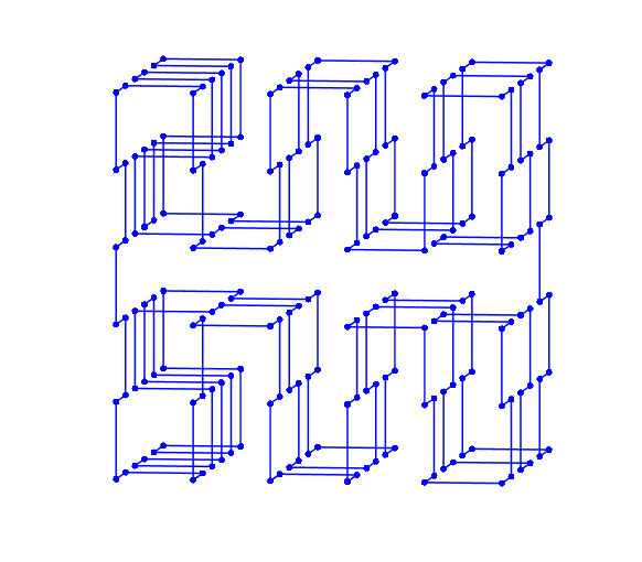
Partial answer: It is possible for $C_n$ if $n$ is a power of two.
$C_2$ and $C_4$ are shown in the question. For larger $n$ the idea is to take a three-dimensional Moore curve (a recursive construction of a Hamiltonian circuit), and fix any straight-edge trouble locally.
By "recursive" I mean the construction breaks the cube into 8 subcubes, recursively, until the smallest cubest are $C_2$.
The key part is the "local fixing". Take a 3D Moore curve on $C_n$ (with $n=2^k$). Look at each of its $C_2$ subcubes. Each such subcube is entered at one corner, and exited at another corner, in some direction. If the path in the subcube turns properly (both immediately after entering, and also immediately before exiting), we are happy with that subcube. Otherwise, we rotate the path in the subcube so that it turns properly. This is a local fix that does not affect any other parts of the Hamiltonian circuit, and fixes any straight-edge trouble associated with that subcube. Do it for all offending subcubes and you are done.
The only remaining question is whether we can always perform such rotations. In fact we can (see below).
Examples
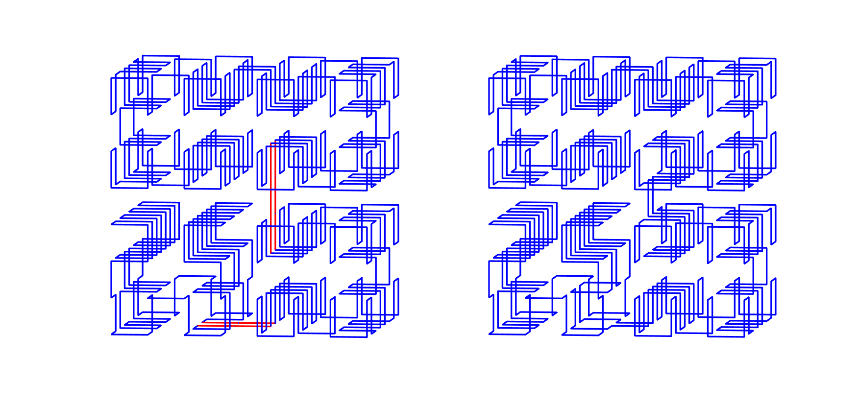
First, a Hamiltonian circuit on $C_8$ before and after fixing. On the left, red edges are defects (consecutive straight edges).
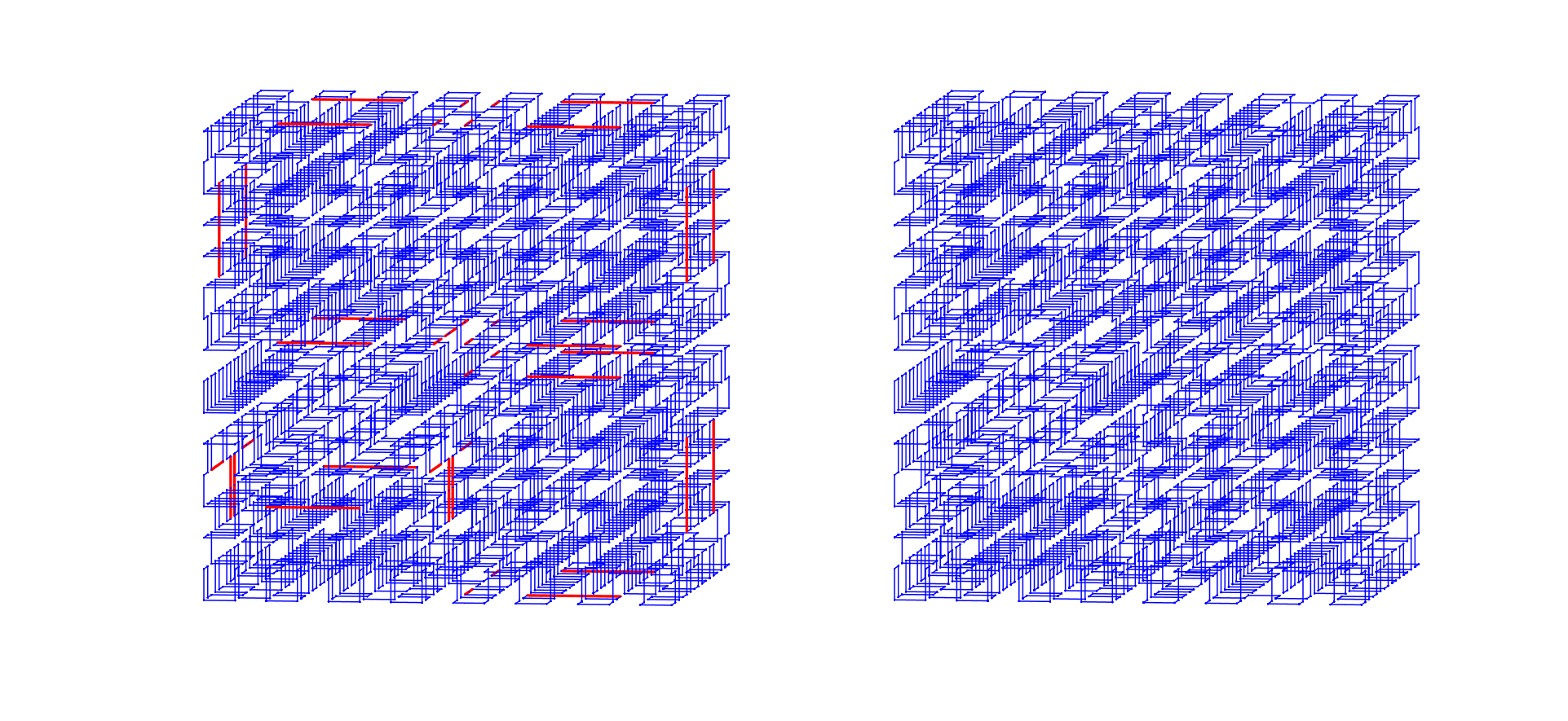
Then the same on $C_{16}$. Of course it is impossible to verify its correctness from the picture, but you get the idea, and the red edges again show the defects, which are fixed on the right.
Details: Recursive construction
First we need a 3D Moore curve (allowing straight-edge defects for the moment). From Wikipedia we learn that you just take eight smaller 3-dimensional Hilbert curves, "rotate them and connect them by line segments". Let's do that carefully. One way to actually do it is with 3-dimensional turtle graphics. We use the following primitives:
- F = forward move one step
- L = left turn
- R = right turn
- U = upward turn ("pitch" if you think of airplane movement)
- D = downward turn
- C = clockwise roll (again, think of an airplane rolling to the right, with nose direction not changing)
- A = anticlockwise roll
Then define some auxiliary terms.
$R(2)$ is a "right-handed" Hamiltonian path on $C_2$. If you place the cube in front of you, you enter the front lower left corner, with your head up. You visit the 8 vertices, and when you exit, you are facing the opposite direction. This can be done with moves UFDFDFRFRFDFDFU.
$L(2)$ is the mirror image of the previous: You enter the cube at its front lower right corner. The moves are UFDFDFLFLFDFDFU.
$R(n)$ is a generic version where you enter a big cube ($n=2^k$ with $n\ge 4$) from the front lower left corner, facing forwards, and exit at front lower right corner, facing back. It is defined as 'C2RF 1LF L1F C2RF R2F A1LF L1F R2A', spaces are just filler for easier reading. If you plug in $R(2)$ for all occurrences of "1", and $L(2)$ for all occurrences of "2", you get a "right-handed" Hamiltonian path on $C_4$. Note that it is not a Hamiltonian circuit since entrance (left corner) and exit (right corner) are far apart.
$L(n)$ is the corresponding generic left-handed Hamiltonian path. The moves are 'A1LF 2RF R2F A1LF L1F C2RF R2F L1C'.
One more: $C(n)$ is a Hamiltonian circuit on a big cube ($C_n$). Its moves are '1LF A1LF L1F 1CRF RA1F 1LF L1F CL1 F'.
Now, for example, you get a circuit on $C_{16}$ by taking the string of $C(n)$, and plugging in $R(8)$ for each occurrence of "1", and $L(8)$ for each occurence of "2".
That gives you a Hamiltonian circuit, but it may have defects.
Fixing the defects
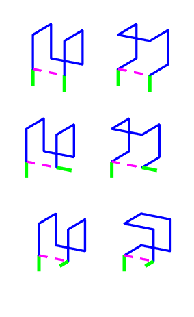
Actually, this is the easier part, but there are a few cases to consider. In the 3D Moore curve, as constructed above, each $C_2$ has the same kind of Hamiltonian path, in some orientation: It contains two parallel "U" curves, joined by an edge. Consider the three cases in this figure. Blue edges show the path inside our cube. Green edges are the entering and exiting edges from an adjacent cube. The magenta dashed line is not part of the path, but it is useful for illustration: it connects the entrance vertex and the exit vertex, and we call it the rod.
- Top left: Both green edges are collinear with the adjoining blue edges. Both defects are fixed by mirroring our curve (top right).
- Middle left: Only one of the green edges is collinear with its blue edge. The other green is collinear with the rod. Again we mirror the curve (middle right).
- Bottom left: Only one of the green edges is collinear with its blue edge. The other green is orthogonal to its blue and to the rod. This is problematic: mirroring does not help. Here we replace our curve with a different Hamiltonian path on the $C_2$ (bottom right).
These cases cover all possible defects, so all defects are locally fixed.
In fact, given the kind of 3D Moore curve described previously, it seems that we never even encounter case 3, at least not up to $C_{256}$, so it seems the mirroring operation is enough! But I did not prove this, so I'm leaving case 3 there "just in case".
The $C_6$ case
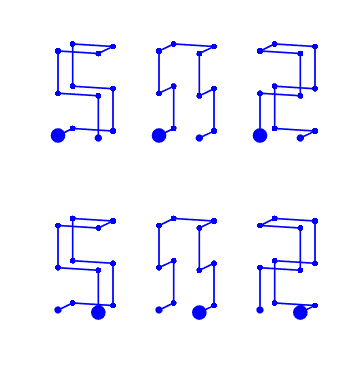
Update: $C_6$ is also possible. We use the following six primitives, each implementing a Hamiltonian path in a $(2 \times 2 \times 3)$ box (big dot indicates entrance). Arranging nine of them suitably, we can fill a $(6 \times 6 \times 3)$ box; this is the top half of our solution. The bottom half is its mirror image.

