This is more an extended comment than an answer.
In my first comment I proposed to rewrite the series $f(x)$ as a series $$\small \begin{eqnarray} g(t)&=& \big ( (1-t )-1 \big) - \big((1-t)^2-1\big) + \big((1-t)^{2^2}-1\big) - ... + ... \\ &=& (-t) - ( -2t+t^2 ) + (-3t+3t^2-t^3 ) -... + ... \end{eqnarray}\tag 1 $$ such that -hopefully- we can write $ \small f(x)=g(1-x) + \frac 12 $ and for example $ \small f(0.99) = g(0.01) + \frac 12 $ by some much smoother evaluatable series.
This ansatz did not solve the problem fully, but gives an interesting detail, which I should possibly ask in a separate question.
I proceeded from eq (1) by formally collecting equal powers of the argument $t$ getting at each power of $t$ an infinite series, which are all divergent, but are compositions of geometric series with alternating sign - and usually we can use the closed forms for this. What I got is the following $$\small \begin{eqnarray} g(t)&=& &(-t)\cdot & ( 1-2+4-8+16-...+...) \\ && + &(-t)^2 \cdot & ( -1 + 6 -28 +120- ... + ...)\\ && + & & ... \\ && + & (-t)^k \cdot & \sum_{j=1}^\infty (-1)^j \binom{2^j}{k} \\ && \vdots \end{eqnarray} \tag 2$$ It is now interesting, that the binomial-series have closed forms, and can exactly be expressed by Stirlingnumbers 1st kind and the closed forms of geometric series with quotients $-(2^k)$ so that for instance the first few coefficients can be written as $$\small \begin{eqnarray} g(t)&=& &(-t)\cdot &\frac 1{1!}& ( + 1{1 \over1+2^1} &&& ) \\ && + &(-t)^2 \cdot &\frac 1{2!}& ( -1{1 \over1+2^1} &+1{1 \over1+2^2}&& ) \\ && + &(-t)^3 \cdot &\frac 1{3!}& (+ 2{1 \over1+2^1} &-3{1 \over1+2^2}&+1{1 \over1+2^3}& ) \\ && \vdots \end{eqnarray} \tag 3$$ If we change order of evaluation now we have columnwise the mercatorseries for $log(1-y)$ and its powers so that we can write $$ \small g(t) = 1/2 + {\log(1-t)\over 1! }{1\over 3} + {\log(1-t)^2\over 2! }{1\over5} + ... \tag 4$$ and finally $$ g(t) = \sum_{k=0}^\infty {\log(1-t)^k\over k! }{1\over 1+2^k} \tag 5$$
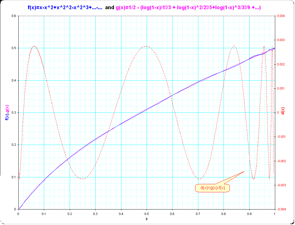
But this decomposition into double series and change order of computations is not yet enough to reproduce $f(x)$. My first impression was that this is a road to nirvana, but now I see, that the error has systematic pattern and thus might possibly be "cured" by one more step: the curve of the differences $d(x) = f(x)-g(x)$
a) has a sinusoidal pattern and -even better -
b) seem to have a constant amplitude.
Here are pictures of the function $f(x)$, $g(1-x)$ and $d(x)= g(1-x)-f(x)$:
 The blue line and the magenta line are nicely overlaid over the whole range $0<x<1$ and the amplitude of the red error-curve (the y-scale is at the right side) seems to be constant.
For the more critical range near $x=1$ I've a zoomed picture:
![[bild2]](https://i.sstatic.net/BqXL6.png) But now I'm missing the tools to proceed. Possibly we have here something like in the Ramnujan-summation where we have to add some integral, don't know.
But now I'm missing the tools to proceed. Possibly we have here something like in the Ramnujan-summation where we have to add some integral, don't know.
But if we have in fact the amplitude of the error (=difference $d(x)$) constant, then a discussion of the (likely) easier series $g(x)$ might allow to infer to the properties of the oscillations in $f(x)$
