Interpolating between piecewise linear functions, with a family of smooth functions

Question

Let $[a,b)\subset\mathbb R$, and $F,G:[a,b)\to\mathbb R$ two decreasing piecewise linear functions so that $F(x)\leq G(x)$ for any $x\in[a,b)$. We assume that:

1. there is a number $k\in\mathbb N-\{0\}$ and a set of $k+1$ numbers $a=x_0\lt\ldots\lt x_k=b$ partitioning $[a,b)$ in $k$ intervals $[x_{j-1},x_j)$ on which the restrictions of $F$ and $G$ are linear.
2. the equalizer set $E=Eq(F,G):=\{x\in[a,b)|F(x)=G(x)\}$ is included in the set $\{x_0,x_1,\ldots,x_k\}$.
3. the restriction of $F$ to the set $E$ is strictly decreasing
4. for any $j$, $0\lt j\lt k$, there is an open neighborhood $(x_j-\epsilon,x_j+\epsilon)$, and a linear function $L:(x_j-\epsilon,x_j+\epsilon)\to\mathbb R$, so that $G\geq L\geq F$ on $(x_j-\epsilon,x_j+\epsilon)$.

(conditions 2-4 forbid some cases when the problem has no solution)

Problem: Find a continuous family of functions $f_t:[a,b)\to\mathbb R$, $t\in[0,1]$ satisfying the conditions:

1. $f_t$ is smooth and strictly decreasing for any $t\in(0,1)$.
2. For any fixed $x\in[a,b)-E$, the application $\vartheta_x:[0,1]\to [F(x),G(x)]$, $\vartheta_x(t)=f_t(x)$ is a strictly increasing and bijective smooth function.

It is easy to see that from the condition 2 it follows that:

• if $0\leq s\lt t\leq 1$, then $f(s)\lt f(t)$ on $[a,b)-E$ (and of course $f(s)=f(t)=F=G$ on $E$).
• $f_0=F$ and $f_1=G$.

If possible, please also provide some references which can help solving this problem.

---

Update 1:

So far I tried to construct the functions from known analytical functions, splines and sigmoids, and to use Schwarz-Christoffel to map the region between $F$ and $G$ to a rectangle in the complex plane. While these methods appeared to have some advantages, it seems difficult to show that they really satisfy the required conditions. Anyway, I don't want to reinvent the wheel.

Answer 1

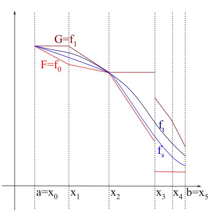
As noted by Dejan Govc, the set $E$ should also contain those points where the right limit of $F(x)$ equals the left limit of $G(x)$, because any continuous function bounded between $F$ and $G$ will be forced to the unique limit in these points.

---

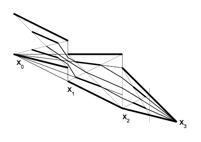
Let's first describe a construction for a family of continuous functions, which will later be refined to give a family of smooth functions. In the picture below, the parts where the smooth construction is identical to the continuous construction are drawn with bold lines. The drawn parts are $f_t(x)$ for $t=\frac{1}{4}$, $t=\frac{1}{2}$ and $t=\frac{3}{4}$. The construction separates an interval into four different regions, either using the diagonal if $F$ and $G$ don't meet each other in the interval, or cutting the interval in half an using the diagonals of the subinterval where $F$ and $G$ don't meet.

The piecewise linear family $p_t(x)=(1-t)F(x)+tG(x)$ corresponds to a family of straight lines inside of each interval. This family either consists of parallel lines, or these lines meet in a common point which is not inside the interval. The bold lines in the image are the parts where we have $f_t(x)=p_t(x)$.

Let $y_j:=\lim_{x\to x_j^-}F(x)$ be the relevant limit of $F$ at $x_j$ and $Y_j:=\lim_{x\to x_j^+}G(x)$ be the relevant limit of $G$. We have $y_j \leq Y_j$. We use $f_t(x_j)=(1-t)y_j+tY_j$. For the continuous construction, these two different parts of the construction are simply connected by straight lines. Let's denote the resulting family by $f_t^{cont}$. It's easy to check that this construction satisfies to requirements of the question, except that $f_t^{cont}$ (and the corresponding $\vartheta_x^{cont})$ is only continuous instead of smooth, and that the set $E$ had to be enlarged as described above.

---

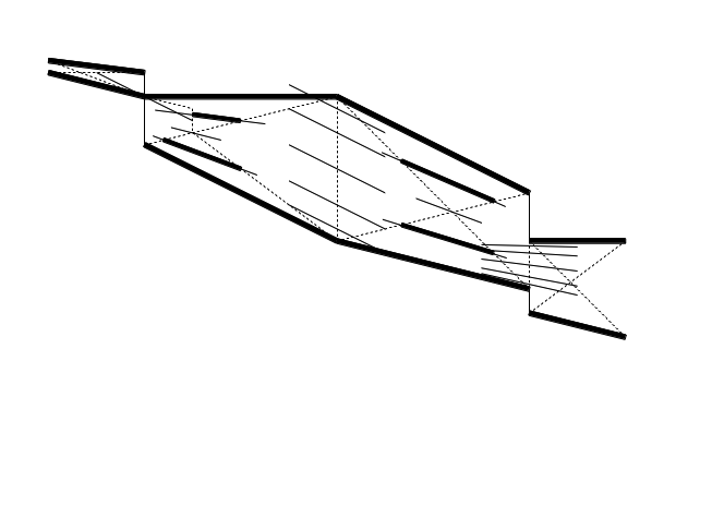
If we want to smooth out the continuous family $f_t^{cont}$ to get a smooth family $f_t$, we need to "specify" how $f_t$ should behave near the non-smooth points of $f_t^{cont}$. It's clear how it should behave near the parts with $f_t(x)=p_t(x)=f_t^{cont}(x)$, so let's focus on the regions around $x_j$. If $y_j < Y_j$, we can use the family of straight lines generated by the straight line given by $F$ on the left side of $x_j$ and by the straight line given by $G$ on the right side of $x_j$. If $y_j=Y_j$, we can use the linear function $L$ from assumption 4 to define how $f_{1/2}$ should behave near $x_j$. Because $f_t$ should not cross $f_{1/2}$, we use $L(x)+(t-\frac{1}{2})x^2$ to define how $f_t$ should behave near $x_j$.

At the left side, we see that line $L$ for the case $y_j=Y_j$ can lead to problems with how we separated the interval into different regions. The image also suggests how these problems can be fixed.

Regarding the missing details of this construction, I had started to explicitly construct the smoothing for the case $y_j < Y_j$, but inadvertently ignored the condition that $\vartheta_x(t)$ should be a smooth function of $t$ instead of just a continuous function. For the case with $y_j=Y_j$, I haven't started to think about an explicit smoothing, and I also don't know for sure whether the behavior of $f_t$ around $x_j$ prescribed above will always allow such a smoothing (but a more "generic" linear function $L$ with strict inequalities should fix this, in case it really is a problem).

---

Regarding references, this is one of the reasons why I decided to work out a detailed solution. A long time ago, I wrote a German text that starts by construction smooth and differential curves satisfying various conditions (these curves are used as "test curves" later in the text). That text cites normal introductory and slightly advanced analysis texts as main references. I really think this is the place where one gets taught how to construct curves adapted to various purposes. It is laborious to do so, but I fear no theory will save us from that.