$\newcommand\ka\kappa\newcommand\la\lambda$Let us show that
\begin{equation*}
\ka(p)=p\quad\text{for }p\in[1/6,1/2]. \tag{1}\label{1}
\end{equation*}
Indeed, suppose that $p\in[1/6,1/2]$. Write
\begin{equation*}
\ka(p) = \sup_{t>0}f_p(t),
\end{equation*}
where
\begin{equation*}
f_p(t):=\frac{\ln(1-2p+2p\cosh t)}{t^2}.
\end{equation*}
For real $t>0$, let
\begin{equation*}
g_p(t):=f'_p(t)\frac{t^3}2=\frac{pt\sinh t}{1-2p+2p\cosh t}-\ln(1-2p+2p\cosh t).
\end{equation*}
Then
\begin{equation*}
\begin{aligned}
h_p(t)&:=g'_p(t)\frac{(1-2p+2p\cosh t)^2}p \\
&=t \cosh t-\sinh t-4 p (t+\sinh t) \sinh ^2\frac t2
\\
& \le h_{1/6}(t)=-\sum_{k\ge2}\frac{2^{2k+1}-8k}{6(2k+1)!}\,t^{2k+1}<0,
\end{aligned}
\end{equation*}
so that $g_p(t)$ is decreasing (in $t>0$). Also, $g_p(0+)=0$. So, $g_p(t)<0$ (for $t>0$) and hence $f_p(t)$ is decreasing (in $t>0$). So,
\begin{equation*}
\ka(p) = f_p(0+)=p,
\end{equation*}
which proves \eqref{1}.
For $p\in(0,1/6]$, a quick bound on $\ka(p)$ can be obtained from the Kearns--Saul inequality -- see e.g. inequality (1.1), which states that the subgaussian constant for a centered Bernoulli random variable (r.v.) $X$ with parameter $r\in(0,1)$ is no greater than (actually, is equal to)
\begin{equation*}
c(r):=\frac{1-2r}{4\ln(1/r-1)}.
\end{equation*}
Note that, if $p\in(0,1/4]$, $X$ is as above, $Y$ is an independent copy of $X$, and $r=r_p:=\frac12-\sqrt{\frac14-p}$, then $X-Y$ will equal your r.v. $\xi$ in distribution. It follows that for $p\in(0,1/6]$
\begin{equation*}
\ka(p)\le2c(r_p). \tag{2}\label{2}
\end{equation*}
On the other hand, by Jensen's inequality for the convex function $y\mapsto e^y$, we have $Ee^{t\xi}=Ee^{t(X-Y)}\ge Ee^{tX}=e^{c(r_p)t^2}$ for some $t>0$ depending on $p$. So,
\begin{equation*}
\ka(p)\ge c(r_p). \tag{3}\label{3}
\end{equation*}
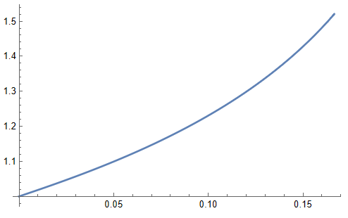
So, by \eqref{2} and \eqref{3}, for all $p\in(0,1/6]$ the subgaussian constant $\ka(p)$ differs from $c(r_p)$ by a factor in the interval $[1,2]$.
This is illustrated by the graph $\Big\{\dfrac{\ka(p)}{c(r_p)}\colon0<p<1/6\Big\}$ below:

Added:
The OP wrote: "My end goal was to bound the expectation of the maximum of $n$ such things with a $\sqrt{\log n}$ dependence" ... What is meant here concerning a $\sqrt{\log n}$ dependence is apparently the following: If $\xi_1,\dots,\xi_n$ are standard normal random variables (r.v.'s), then
\begin{equation*}
E\max_1^n\xi_i=O(\sqrt{\ln n}), \tag{4}\label{4}
\end{equation*}
and, moreover, $E\max_1^n\xi_i\asymp\sqrt{\ln n}$ if $\xi_1,\dots,\xi_n$ are independent standard normal r.v.'s.
However, in contrast with the normal distribution, for small $p$ the distribution of the r.v. $\xi$ as in the OP has rather heavy tails (say in the sense that the absolute moments of $\xi$ grow relatively fast). So, the very slow growth of the expected maximum (as in \eqref{4}) will not be the case with these heavy tails. E.g., if $X_1,\dots,X_n$ are independent copies of the standardized r.v. $\xi$ in distribution, then
\begin{equation*}
E\max_1^n X_i=\frac{1-(1-p)^n-p^n}{\sqrt{2p}}
\sim n\sqrt{p/2} \quad \\
\text{if $n\to\infty$ and $np\to0$,} \tag{5}\label{5}
\end{equation*}
so that $E\max_1^n X_i$ grows asymptotically linearly with $n$ in this regime.
If now $n\to\infty$ and $np\to\la\in(0,\infty)$ (the symmetrized Poisson regime), then $E\max_1^n X_i\sim C_\la\, \sqrt n$ with $C_\la:=(1-e^{-\la})/\sqrt{2\la}$, still a much faster rate of growth than $\sqrt{\ln n}$. We can also write
\begin{equation*}
E\max_1^n X_i
\sim C_\la n\sqrt{p/\la} \quad\text{if $n\to\infty$ and $np\to\la\in(0,\infty)$}. \tag{6}\label{6}
\end{equation*}
All this indicates that it is not a good idea to use a (sub)Gaussian bound for the distribution of the r.v. $\xi$ as in the OP if $p$ is small. Instead, letting then $X_1,\dots,X_n$ be any (not necessarily independent) copies of the standardized r.v. $\xi$ in distribution, we can simply write
\begin{equation*}
E\max_1^n X_i\le E\sum_1^n \max(0,X_i)=n\sqrt{p/2},
\end{equation*}
which agrees well with the independent-case asymptotics in \eqref{5} and \eqref{6}.

