Singular Fisher information matrix and existence of unbiased estimators

Question

I'm doing some research into the Cramer-Rao bound for time of arrival localization and have come across a rather strange result: the FIM is singular, but there exists an unbiased estimator. My supervisor insists I'm wrong (I'm sure I must be), but I can't seem to figure out what I'm doing wrong. Can someone please help guide me in the right direction? Sorry for the long development of the problem below.

---

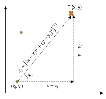
A transmitter $T$ is at an unknown location $\theta=(x, y)^T$. There are $s$ sensors in the region $\Omega$. The $j^\text{th}$ sensor positioned at $\theta_j=(x_j, y_j)^T$ measures a range to $T$ that is a random variable dependent on the actual distance of $T$ from the sensor ($d_j$), as shown below:

The range measurement vector for all anchors is therefore: $$ r = [d_1 + \varepsilon_1, \ldots, d_j + \varepsilon_j]^T = d(\theta)+\varepsilon=\|\theta-\theta_j\|_2 + \varepsilon $$

where the error is assumed to be normally distributed $\epsilon \sim N\left(0, \Sigma_{s_{\mathrm{x}}s} \right)$.

For a multivariate Gaussian distribution, the $(m,n)$ element of the FIM is:

$$ FIM_{m,n}=\frac{\partial d^T}{\partial \theta_m} \Sigma^{-1} \frac{\partial d}{\partial \theta_n}+\frac{1}{2} \operatorname{TR}\left(\Sigma^{-1} \frac{\partial \Sigma}{\partial \theta_m} \Sigma^{-1} \frac{\partial \Sigma}{\partial \theta_n}\right) $$

Assuming independent noise at the sensor measurement and a constant variance for the noise at each sensor, the covariance matrix is diagonal, i.e. $\Sigma=\operatorname{diag}(\sigma^2_1, \sigma^2_2,\ldots, \sigma^2_s)$. Thus, the FIM can be expanded for $\theta=(x, y)^T$ as:

\begin{equation} \left[\begin{array}{cc} FIM_{1,1} & FIM_{1,2} \\ FIM_{2,1} & FIM_{2,2} \end{array}\right] \end{equation}

\begin{align} \label{FIM11} FIM_{1,1} &= \sum_{j=1}^s \frac{1}{2} \left(\sigma_j^2\right)^{-2} \left(\frac{\partial \sigma_j^2}{\partial x} \right)^2 + \left(\sigma_j^2\right)^{-1}\left(\frac{\partial d_j}{\partial x}\right)^2 \\ & = \sum_{j=1}^s \left(\sigma_j^2\right)^{-1} \cos^2 (\phi_j) \end{align}

\begin{align} \label{FIM12} FIM_{1,2}=FIM_{2,1}&=\sum_{j=1}^{s} \frac{1}{2} \left(\sigma_j^2\right)^{-2} \frac{\partial \sigma_j^2}{\partial x} \frac{\partial \sigma_j^2}{\partial y} + \left(\sigma_j^2 \right)^{-1} \frac{\partial d_j}{\partial x} \frac{\partial d_j}{\partial y}\\ &=\sum_{j=1}^s \left(\sigma_j^2 \right)^{-1} \cos(\phi_j) \sin(\phi_j) \end{align}

\begin{align} \label{FIM22} FIM_{2,2} &= \sum_{j=1}^s \frac{1}{2}\left(\sigma_j^2 \right)^{-2} \left(\frac{\partial \sigma_j^2}{\partial y}\right)^2 + \left(\sigma_j^2 \right)^{-1} \left(\frac{\partial d_j}{\partial y}\right)^2 \\ &=\sum_{j=1}^s \left(\sigma_j^2 \right)^{-1} \sin(\phi_j)^2 \end{align}

where $\phi_j$ is the angle between the $j^\text{th}$ sensor and T, since

\begin{align} \frac{\partial d_{j}}{\partial x}&=\frac{\partial}{\partial x} \left[(x-x_j)^{2}+(y-y_j)^{2}\right]^{\frac{1}{2}}=(x-x_j)d_{j}^{-1}\\ &=cos(\phi_j) \end{align}

And similarly $\frac{\partial d_j}{\partial y}=sin(\phi_j)$.

Consider three sensors situated at $(-1,0),$ $(0,0)$ and $(1,0),$ and $T$ at $(2,0).$ The FIM is clearly singular as $\phi_j=0 \, \forall j$ and so the CRB does not exist. The negative log-likelihood function (NLL) can be written as:

\begin{align} -\mathcal{L}&=-\log\left(\prod_{j=1}^{s} P_{r}\left(r_{j} ; d_{j}\right)\right) = -\log\left(\prod_{j=1}^{s} \frac{1}{\sqrt{2 \pi \sigma_{j}^{2}}} e^{-\frac{\left(r_{j}-d_{j}\right)^{2}}{2 \sigma_{j}^{2}}}\right)\\ &= \sum_{j=1}^{s}\left[\frac{1}{2}\log (2 \pi)+\frac{1}{2} \log \left(\sigma^{2}_{j}\right)+\frac{(r-d_{j})^{2}}{2 \sigma^{2}_{j}}\right] \end{align}

I've done an MLE simulation in MATLAB for this.

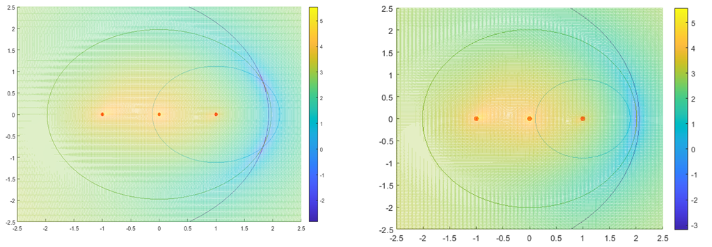
The circles for two different range measurements vectors are shown below, overlayed with the negative log-likelihood (NLL) function for the measurement.

There are two situations that happen with the range circles:

1. When 2 or more circles intersect, they do so at two locations (the two bluish regions in the left plot) which have reflection symmetry along the $y=0$ line, and so the NLL function has a minima at these two points.

2. When no circles intersect, the NLL function has a minima on the $y=0$ line (think of this in a least-squares sense: when the circles don't intersect, the least squares estimate is where they are closest, which is the bluish region in the right plot).

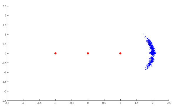
Therefore, the $y$-coordinate MLE (i.e. estimator that minimizes NLL function) is unbiased and has finite variance.

This is the output of 1500 MLE estimates I computed in a simulation:

I can't seem to figure out where I've gone wrong.

EDIT: I asked this question in math.stackexchange, but I figure this is probably a better place to ask it since it's PhD research that I'm doing. Also as background, I'm an engineer but part of my supervisory team looking at this part of my work is composed of mathematicians.

Answer 1

$\newcommand\th\theta\newcommand\ol\overline$Responsding to your comments:

"About the collinear sensors in my question: I understand that for $y\ne0$, the model is non-identifiable. But, what I find unusual is that for $y\ne0$, the Fisher information matrix is full rank, but at the only $y$-coordinate value where the model is identifiable (i.e. $y=0$), the Fisher information matrix is singular.

And further, at $(x,0)$, the $y$-coordinate MLE is asymptotically unbiased, even though the Fisher information matrix is singular at $(x,0)$.

All this is the consequence of the simple fact that, for collinear sensors, $(x,y)$ is a wrong choice of a parameter, because then the model is not identifiable.

To illustrate this, here is a simpler model that exhibits all the features that confused you. Let $X_1,\dots,X_n$ be independent $N(\th^2,1)$ random variables, where the parameter $\th$ may take any real value. Similarly to your model, the latter, simpler model is "identifiable only at $\th=0$". Also similarly to your model, in the simpler model the $1\times1$ Fisher information matrix is singular only at $\th=0$.

Only $\th^2$ is identifiable and estimable in the simpler model, just as only $(x,y^2)$ is identifiable and estimable in your collinear-sensors model. The MLE of $\th^2$ in the simpler model if $\widehat{\th^2_n}=\max(0,\ol X_n)$, where $\ol X_n:=\frac1n\,\sum_{i=1}^n X_i$. Similarly to your model, in the simpler model the estimators $\pm\sqrt{\widehat{\th^2_n}}=\pm\sqrt{\max(0,\ol X_n)}$ are "consistent and asymptotically unbiased at $\th=0$", in the sense that $\pm\sqrt{\widehat{\th^2_n}}\to0$ in probability and $\pm E\sqrt{\widehat{\th^2_n}}\to0$ as $n\to\infty$ if $\th=0$ is the true value of the parameter.

---

Summarizing, we can say again that the cause of all the confusion is that, for collinear sensors, $(x,y)$ is a wrong choice of a parameter. Letting, for collinear sensors, $(x,u)$ be the parameter with $u:=y^2$, we get an identifiable model, with an everywhere non-singular Fisher information matrix.