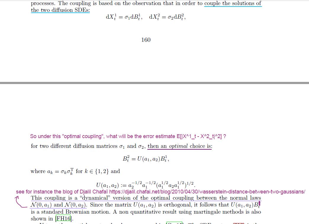
Take $\sigma_1 = a_1^{1/2}$ and $\sigma_2 = a_2^{1/2}$. Consider the coupling
$$ X^1_t = X_0^1 + a_1^{1/2} B^1_t \quad \text{and} \quad X^2_t = X_0^2 + a_2^{1/2} U(a_1, a_2) B_t^1 \;.
$$ Here $U(a_1,a_2) = a_2^{-1/2} a_1^{-1/2} (a_1^{1/2} a_2 a_1^{1/2} )^{1/2}$ is an orthogonal matrix since $$
U(a_1,a_2) U(a_1, a_2)^T = a_2^{-1/2} a_1^{-1/2} (a_1^{1/2} a_2 a_1^{1/2} ) a_1^{-1/2} a_2^{-1/2} = I
$$ where $I$ is the identity matrix. As a shorthand, let $A =a_1^{1/2} - a_2^{1/2} U(a_1, a_2) $, so that
$$
X_t^1 - X_t^2 = X_0^1 - X_0^2 + A B_t^1 \;.
$$
Then
\begin{align}
E[|X^1_t - X^2_t|^2] &= |X_0^1 - X_0^2|^2 + E[| A B^1_t|^2] = |X_0^1 - X_0^2|^2 + E[(A B^1_t)^T (A B^1_t)] \\
&= |X_0^1 - X_0^2|^2 + E[\operatorname{Trace}( ( A B^1_t)^T (A B^1_t)) ] \\
&= |X_0^1 - X_0^2|^2 + E[\operatorname{Trace}( A (B^1_t) (B^1_t)^T A^T ) ] \\
&= |X_0^1 - X_0^2|^2 + t \operatorname{Trace}( A A^T )
\end{align}
where we used the cyclic property of the trace and the fact that $E[ (B^1_t) (B^1_t)^T]= t I$.
To finish, \begin{align}
&\operatorname{Trace}( A A^T ) = \operatorname{Trace}( (a_1^{1/2} - a_2^{1/2} U(a_1, a_2)) (a_1^{1/2} - a_2^{1/2} U(a_1, a_2))^T ) \\
&= \operatorname{Trace}( a_1 - a_2^{1/2} U(a_1, a_2) a_1^{1/2} - a_1^{1/2} U(a_1, a_2)^T a_2^{1/2} + a_2^{1/2} U(a_1, a_2) U(a_1, a_2)^T a_2^{1/2} ) \\
&= \operatorname{Trace}( a_1 - 2 a_1^{1/2} a_2^{1/2} U(a_1, a_2) + a_2 ) \\
&= \operatorname{Trace}( a_1 - 2 (a_1^{1/2} a_2 a_1^{1/2} )^{1/2} + a_2 )
\end{align}
where again we used the cyclic property of the trace and that $U(a_1,a_2)$ is an orthogonal matrix. Combining the above we obtain
$$
E[|X^1_t - X^2_t|^2] = |X_0^1 - X_0^2|^2 + t \operatorname{Trace}( a_1 + a_2 - 2 (a_1^{1/2} a_2 a_1^{1/2} )^{1/2} ) \;,
$$ as required. This is indeed a dynamical (i.e., time-dependent) version of the 2-Wasserstein distance between two multivariate normal distributions.
In contrast, for the synchronous coupling,
$$
X^1_t = X_0^1 + a_1^{1/2} B^1_t \quad \text{and} \quad X^2_t = X_0^2 + a_2^{1/2} B_t^1 \;,
$$ we obtain:
$$
E[|X^1_t - X^2_t|^2] = |X_0^1 - X_0^2|^2 + t \operatorname{Trace}( a_1 + a_2 - 2 a_1^{1/4} a_2^{1/2} a_1^{1/4} ) \;.
$$
As discussed further in Section 2 of the reference below, we note that the synchronous coupling is optimal with respect to the 2-Wasserstein distance when $a_1$ and $a_2$ commute, since in that case $U(a_1,a_2)=I$.
Givens, Clark R.; Shortt, Rae Michael, A class of Wasserstein metrics for probability distributions, Mich. Math. J. 31, 231-240 (1984). ZBL0582.60002.

