Example of a differentiable function optimization where derivative free methods are used

Question

While preparing a workshop on the derivative free methods, and fminsearch in MATLAB, I found an example function where fminsearch converges better and in less iterations than fmincon with calculated derivatives. Since fminsearch uses Nelder-Mead method, I suppose it would do a better job in terms of optimization, when a function has a lot of variables, but is quadratic.

Do you happen to know any concrete examples of a function or a class of differentiable functions where calculating the derivatives doesn't help optimization-wise?

Any answer would be really useful.

Answer 1

I suppose one general situation where Nelder-Mead might perform better is when the objective function is 'simple' at the length scale of the initial simplex, but is very oscillatory at the 'microscopic' scale; in this sort of situation, Nelder-Mead won't 'see' the complicated local behaviour, whereas a derivative-based method could be confused and impeded by it.

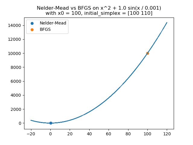
For a concrete example on the real line, I had a play at finding the global minimum of $x\longmapsto x^2 + \sin(1000 x)$ with different initial conditions and marked the minima found by Nelder-Mead (blue dot) and BFGS (orange dot).

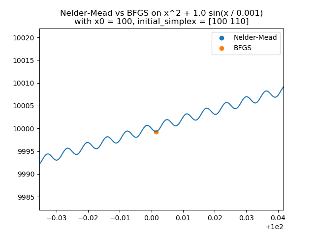
Zooming in to look at what went wrong for BFGS, it seems pretty likely that it's been thwarted by the 'microscopic' oscillations:

I've included the Python 3 code used to generate the plots in case that's helpful. The script below receives an amplitude and a wavelength as positional arguments when run from the command-line.

"""
Script for illustrating one situation when derivative-based optimisation methods can get into trouble.
"""

import matplotlib.pyplot as plt
import numpy as np
import sys
from scipy.optimize import minimize

# Read inputs from command line
amplitude = float(sys.argv[3])  # e.g. 1.0
wavelength = float(sys.argv[4])  # e.g. 1.0e-3

# Set up objective function and its derivative
objective = lambda x: np.square(x) + amplitude * np.sin(x / wavelength)
derivative = lambda x: 2 * x + (amplitude / wavelength) * np.cos(x / wavelength)

# Set up a starting position and a large initial simplex
starting_position = 100
initial_simplex_length = 10
initial_simplex = np.array([
    [starting_position],
    [starting_position + initial_simplex_length]
])

# Minimise using NM
results = {}
results["Nelder-Mead"] = minimize(
    objective,
    starting_position,
    method="Nelder-Mead",
    options={
        "initial_simplex": initial_simplex
    }
)

# Minimise using BFGS
results["BFGS"] = minimize(
    objective,
    starting_position,
    method="BFGS",
    jac=derivative
)

# Initialise plot
_, ax = plt.subplots()

# Plot objective function
xs = np.arange(-0.2 * starting_position, 1.2 * starting_position, 0.5 * wavelength)
ax.plot(xs, objective(xs))

# Mark minima found by both methods
for method, result in results.items():
    ax.scatter(
        [np.squeeze(result.x)],
        [result.fun],
        label=method
    )

ax.legend()
ax.set_title(
    f"Nelder-Mead vs BFGS on x^2 + {amplitude} sin(x / {wavelength})\n"
    f"with x0 = {starting_position}, initial_simplex = {np.squeeze(initial_simplex)}"
)
plt.show()

# Print results
print(results)