Does the plane clustered to minimize sum distances^2 to clusters centers ( inertia / "K-means") produce hexagonal clusters / hexagonal lattice?

Question

"K-means" is the most simple and famous clustering algorithm, which has numerous applications. For a given as an input number of clusters it segments set of points in R^n to that given number of clusters. It minimizes the so-called "inertia" i.e. sum distances^2 to clusters centers = $\sum_{i ~ - ~ cluster~ number} \sum_{X - points~ in ~i-th ~ cluster} |X_{in ~ i-th ~ cluster} - center_{i-th~ cluster} |^2 $

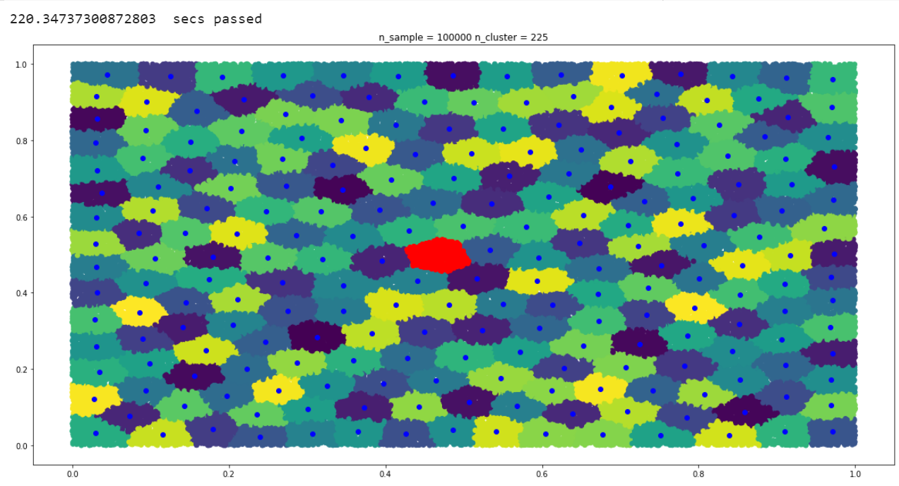
By some reasons let me ask, what happens for the plane i.e. there is no any natural clusters, but still we can pose minimization task and it will produce something. Let us look on the example:

So, most clusters look like hexagons. Especially the most central one which is colored in red. Well, boundary spoils things, also may be not enough sample size/iteration number - simulation is not a perfect thing - but I made many and pictures are similar...
Hexagonal lattice appears in many somewhat related topics, so it might be that some reason exists.

Question 0 What is known on "inertia" minimization on the plane/torus ? (torus - to avoid boundary effects.) (Any references/ideas are welcome). Do hexagons arise as generic clusters ?

Question 1 Consider a torus of sizes R1,R2 , consider the number of clusters to be mn , is it true that hexagonal lattice will provide the global minima for "inertia" ? (At least for consistent values of R1, R2, m,n (R1=am, R2 = a*n) ).

(Instead of finite number of points we can consider the continuous case and substitute summation over points by the integral. Or we can sample large enough uniform datacloud - as done in simulation).

---

Let me mention beautiful survey by Henry Cohn at ICM2010, where lots of optimization problems of somewhat related spirit are discussed and which sound simple, but remain unsolved for years (see also MO78900). That question is not discussed there unfortunately.

The Python code for the simulation above. One can use colab.research.google.com - to run it - no need to install anything - can use google's powers for free.

from sklearn.cluster import  KMeans
import numpy as np
import matplotlib.pyplot as plt
from scipy.spatial.distance import cdist
import time
#import datetime

t0 = time.time()
N = 10**5 # Number of uniformly scattered point 
d = 2 # dimension of space 
X = np.random.rand(N,d) # Generate random uniform N poins on [0,1]^d
n_clusters = 225 # Number of clusters for Kmeans
clustering = KMeans(n_clusters=n_clusters,  
      init='k-means++', n_init=10, max_iter=600, # max_iter increased twice from default  
      tol=0.0001,  random_state=None,  algorithm= 'full' ).fit(X) # Run K-means with default params 
      # https://scikit-learn.org/stable/modules/generated/sklearn.cluster.KMeans.html#sklearn.cluster.KMeans

print(time.time() - t0, ' secs passed' ) # Print time passed 

cluster_centers_ = clustering.cluster_centers_ # 
predicted_clusters = clustering.labels_ #

####################################################################
# Choose the most central classter - hope boundary effect on it would be negligble 
central_point = 0.5 * np.ones(d)  # Choose central pint  
idx_most_central_cluster  = np.argmin( cdist( central_point.reshape(1,-1), cluster_centers_ ) ) # Find cluster most close to central point 
coords_most_central_cluster_center = cluster_centers_[idx_most_central_cluster,: ] 
mask = idx_most_central_cluster  == predicted_clusters 
Xm = X[mask,: ] # Select only points from the most central cluster

#######################################################################
# Plotting 
fig = plt.figure( figsize= (20,10 ) ) # 20 - horizontal size, 6 - vertical size 
plt.scatter( X[:,0], X[:,1], c = predicted_clusters )  # scatter plot all the points  colored according to different clusters
plt.scatter( cluster_centers_[:,0],  cluster_centers_[:,1], c = 'blue' ) # Mark centers of the clusters
plt.scatter( Xm[:,0], Xm[:,1], c = 'red' ) # Color by red most central cluster 
plt.title('n_sample = '+str(N) + ' n_cluster = ' + str(n_clusters))
plt.show() 

Answer 1

The answer is yes, at least in the limiting case where the number of points tends to infinity.

Specifically, this is known as the quantizer problem (see Chapter 2 of Sphere Packings, Lattices and Groups by Conway and Sloane). The two-dimensional version of the problem was solved by Fejes Tóth, who showed that the hexagonal lattice is optimal.

László Fejes Tóth, 1959: Sur la représentation d'une population infinie par un nombre fini d'éléments

The way that the quantizer problem is formalised in Sphere Packings, Lattices and Groups is to take a large compact ball $B \subsetneq \mathbb{R}^n$ and ask for the limit (as $M \rightarrow \infty$) of the infimum (over all arrangements of $M$ points in the ball) of the normalised mean squared error from a uniform random point in the ball to the closest of the $M$ points:

$$ \dfrac{1}{n} \dfrac{\frac{1}{M} \sum\limits_{i=1}^{M} \int\limits_{V(P_i)} \lVert x - P_i \rVert^2 \; dx}{\left( \frac{1}{M} \sum\limits_{i=1}^{M} \textrm{Vol}(V(P_i)) \right)^{1 + \frac{2}{n}}} $$

Here, $V(P_i) \subseteq B$ is the Voronoi cell of $P_i$. The connection with $k$-means (where $k = M$ and the ambient dimension is $n$) is that the minimiser of this expression must have each $P_i$ be the centroid of its Voronoi cell $V(P_i)$, and therefore the optimal solution is a fixed point of the $k$-means iteration. The complicated normalisation is to ensure that the limit is sensible (e.g. not $0$ or $\infty$).

For $n = 2$, the limit as $M \rightarrow \infty$ of the infimum of the above expression is $\frac{5}{36 \sqrt{3}} \approxeq 0.0801875$, and is the same as the limit as $M \rightarrow \infty$ of the expression where the points are centred at the vertices of a hexagonal lattice (scaled to have exactly $M$ points inside $B$).

For $n = 3$, the best lattice is the body-centred cubic lattice, but there are more efficient nonlattice arrangements and the quantizer problem is unsolved.

In higher dimensions the problem is unsolved.