Why do some linear cellular automata over $Z_{2}$ on the torus have small order?

Question

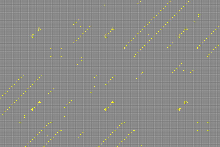
At https://dmishin.github.io/js-revca/index.html, you can play around with reversible cellular automata. I noticed that on that site, that for the reversible linear cellular automata (which I have tested), there is always a small natural number $p$ ($p\leq 12$ in the cases which I have tested) where if the grid is a torus whose dimensions are $2^{n}\times 2^{n}$, then when one runs the cellular automaton $p\cdot 2^{n}$ times, the resulting pattern is the identity function. In other words, if $A$ is the matrix for the linear transformation computing the cellular automaton, then $A^{p\cdot 2^{n}}=I_{2^{2n}}$ but $A^{r}\neq I_{2^{2n}}$ whenever $0<r<p\cdot 2^{n}$.

What is the mathematical explanation of this phenomenon? How pervasive is this phenomena of low periods?

Many of these rules have some sort of Sierpinski triangle pattern, but some have more complicated patterns.

For example, for the rule 0,12,10,6,3,15,9,5,11,7,1,13,8,4,2,14, we apparently have p=7.

Answer 1

Since nobody's posted a full answer yet, let me, for the record, provide my partial answer below. I originally started writing this draft confident that I had the answer, since I was quite familiar with similar phenomena in ordinary linear two-state CA, but then I hit a snag right at the end. Maybe you or someone else can pick up the argument from where I got stuck, though, or at least find something of use in it.

---

If I understand you correctly, you're looking at a subset of two-state Margolus-type block cellular automata that are both reversible (in the sense that the block transition map is bijective) and linear (in the sense that, with the block state space viewed as a vector space over F₂, the transition maps are linear maps).

Let's first look at the behavior of such CA on a 2×2 toroidal lattice (that being the smallest lattice where the Margolus neighborhood makes sense). In this case, the entire lattice consist of a single block. Here it's convenient to assume that, instead of the block boundaries alternating between time steps, the entire lattice configuration is shifted one step diagonally after each time step — which, on a 2×2 cell toroidal lattice, is equivalent to rotating it by 180°.

In this way, we can directly read the time evolution of any configuration of cells on the 2×2 lattice from the block transition table, if we just rotate all the outputs configurations by 180°. For example, for your example automaton on a 2×2 lattice, the single-cell initial configurations evolve as follows:

$$ \substack{\blacksquare \square \\ \square \square} \mapsto \substack{\blacksquare \blacksquare \\ \square \square} \mapsto \substack{\square \blacksquare \\ \blacksquare \square} \mapsto \substack{\blacksquare \square \\ \square \blacksquare} \mapsto \substack{\square \blacksquare \\ \blacksquare \blacksquare} \mapsto \substack{\square \square \\ \blacksquare \square} \mapsto \substack{\square \square \\ \blacksquare \blacksquare} \mapsto \substack{\blacksquare \square \\ \square \square} \\ \substack{\square \blacksquare \\ \square \square} \mapsto \substack{\blacksquare \square \\ \blacksquare \square} \mapsto \substack{\blacksquare \blacksquare \\ \blacksquare \blacksquare} \mapsto \substack{\blacksquare \blacksquare \\ \blacksquare \square} \mapsto \substack{\square \blacksquare \\ \square \blacksquare} \mapsto \substack{\square \square \\ \square \blacksquare} \mapsto \substack{\blacksquare \square \\ \blacksquare \blacksquare} \mapsto \substack{\square \blacksquare \\ \square \square} \\ \substack{\square \square \\ \blacksquare \square} \mapsto \substack{\square \square \\ \blacksquare \blacksquare} \mapsto \substack{\blacksquare \square \\ \square \square} \mapsto \substack{\blacksquare \blacksquare \\ \square \square} \mapsto \substack{\square \blacksquare \\ \blacksquare \square} \mapsto \substack{\blacksquare \square \\ \square \blacksquare} \mapsto \substack{\square \blacksquare \\ \blacksquare \blacksquare} \mapsto \substack{\square \square \\ \blacksquare \square} \\ \substack{\square \square \\ \square \blacksquare} \mapsto \substack{\blacksquare \square \\ \blacksquare \blacksquare} \mapsto \substack{\square \blacksquare \\ \square \square} \mapsto \substack{\blacksquare \square \\ \blacksquare \square} \mapsto \substack{\blacksquare \blacksquare \\ \blacksquare \blacksquare} \mapsto \substack{\blacksquare \blacksquare \\ \blacksquare \square} \mapsto \substack{\square \blacksquare \\ \square \blacksquare} \mapsto \substack{\square \square \\ \square \blacksquare} $$

Since your automata are reversible, all patterns must eventually cycle back to their original state, as seen above. Since your automata are also linear, adding together any two patterns (modulo 2) and letting the resulting pattern evolve simply yields the sum (modulo 2) of the corresponding time evolutions of the original patterns.

As a result, the time evolution of any pattern must return to its original state after $p_1$ steps, where $p_1$ is the least common multiple of the periods of the single-cell patterns. In particular, for your example automaton this period is 7 steps, as shown by the diagram above.

(Note that, if the 2×2 lattice period $p_1$ obtained by the method above is odd, then using the standard Margolus block division scheme with alternating block grids will cause the pattern after $p_1$ steps to be flipped 180° compared to the original pattern, so that $2p_1$ steps are actually needed for the original pattern to reappear exactly. This should not affect the further analysis of 4×4 and larger grids in any substantial way, so I'll ignore that particular detail below.)

---

Now, given that the time evolution of the automaton on a $2^n \times 2^n$ lattice recurs after $p_n$ steps (which it of course, due to reversibility, must do for some period $p_n$), let's consider the same automaton on a $2^{n+1} \times 2^{n+1}$ lattice. Here, it's natural and useful to divide the $2^{n+1} \times 2^{n+1}$ lattice into four $2^n \times 2^n$ quadrants, like this:

\begin{array}{|c|c|} \hline A & B \\ \hline C & D \\ \hline \end{array}

and to look at the evolution of those quadrants over $p_n$ steps.

Since the automata we're considering are all linear, we can limit ourselves to considering the evolution of patterns that are initially confined to, say, the upper left quadrant $A$; the evolution of more complicated initial patterns follows from this by linearity and shift invariance. (Indeed, we could even restrict ourselves to only considering initial patterns consisting of a single live cell in one of the four upper left corner cells, but for the argument given below we don't really need to be that restrictive.)

Let the initial pattern in the upper left $2^n \times 2^n$ quadrant, represented as a $2^{n^2}$-element vector over $\mathbf F_2$, be $\vec x$. By linearity, the patterns in the four quadrants after $p_n$ time steps will then corespond to the vectors $\vec y_A = \mathbf A \vec x$, $\vec y_B = \mathbf B \vec x$, $\vec y_C = \mathbf C \vec x$ and $\vec y_D = \mathbf D \vec x$, where $\mathbf A$, $\mathbf B$, $\mathbf C$ and $\mathbf D$ are some $2^{n^2} \times 2^{n^2}$ matrices that together describe the time evolution of the automaton over $p_n$ steps on the $2^{n+1} \times 2^{n+1}$ cell lattice. Since we know that the same automaton on a $2^n \times 2$ lattice is periodic with period $p_n$, it follows from linearity that $\vec y_A + \vec y_B + \vec y_C + \vec y_D = \vec x$. And since this holds for any initial configuration $\vec x$, we in fact have:

$$\mathbf A + \mathbf B + \mathbf C + \mathbf D = \mathbf I,$$

where $\mathbf I$ is the $2^{n^2} \times 2^{n^2}$ identity matrix.

Given this, let's run the automaton another $p_n$ steps further to obtain the quadrant configurations:

\begin{aligned} \vec z_A &= \mathbf A \vec y_A + \mathbf B \vec y_B + \mathbf C \vec y_C + \mathbf D \vec y_D, \\ \vec z_B &= \mathbf B \vec y_A + \mathbf A \vec y_B + \mathbf D \vec y_C + \mathbf C \vec y_D, \\ \vec z_C &= \mathbf C \vec y_A + \mathbf D \vec y_B + \mathbf A \vec y_C + \mathbf B \vec y_D, \\ \vec z_D &= \mathbf D \vec y_A + \mathbf C \vec y_B + \mathbf B \vec y_C + \mathbf A \vec y_D. \end{aligned}

By substituting in the expressions for $\vec y_A$, $\vec y_B$, $\vec y_C$ and $\vec y_D$ given above, we get:

\begin{aligned} \vec z_A &= (\mathbf A^2 + \mathbf B^2 + \mathbf C^2 + \mathbf D^2) \vec x, \\ \vec z_B &= (\mathbf B \mathbf A + \mathbf A \mathbf B + \mathbf D \mathbf C + \mathbf C \mathbf D) \vec x, \\ \vec z_C &= (\mathbf C \mathbf A + \mathbf D \mathbf B + \mathbf A \mathbf C + \mathbf B \mathbf D) \vec x, \\ \vec z_D &= (\mathbf D \mathbf A + \mathbf C \mathbf B + \mathbf B \mathbf C + \mathbf A \mathbf D) \vec x. \end{aligned}

Now, here's the missing part: if the matrices $\mathbf A$, $\mathbf B$, $\mathbf C$ and $\mathbf D$ all commute with each other, then (given that $1+1=0$ in $\mathbf F_2$) the last three expressions all simplify to $\vec z_B = \vec z_C = \vec z_D = 0$. Meanwhile, the first expression can be rewritten using the same properties as:

\begin{aligned} \vec z_A &= (\mathbf A^2 + \mathbf B^2 + \mathbf C^2 + \mathbf D^2) \vec x \\ &= (\mathbf A + \mathbf B + \mathbf C + \mathbf D)^2 \vec x & (!) \\ &= I^2 \vec x = \vec x. \end{aligned}

(Yes, the square of the sum indeed does equal the sum of the squares here, as can be confirmed by writing it out and observing that all the cross terms cancel out due to the assumed commutativity and cancellation properties noted above.)

---

Unfortunately, I have not been able to show that the matrices $\mathbf A$, $\mathbf B$, $\mathbf C$ and $\mathbf D$ indeed do commute. If we were dealing with an ordinary, fully shift-invariant CA over $\mathbf F_2$, then I believe I could show this by appealing to the shift-invariance and the basic fact that addition of cell coordinates modulo $2^{n+1}$ commutes. But the Margolus lattice is only invariant with respect to shifting by an even number of cells, and that messes things up.

In particular, for a fully shift-invariant CA, knowing that a cell at position $x$ gives rise $p_n$ steps later to a cell at $y = y+\delta_1$, which in turn gives rise $p_n$ steps later to a cell at $z = y+\delta_2 = x+\delta_1+\delta_2$, would imply that the same cell at $x$ must also give rise to a cell at $y' = x+\delta_2$, which must then give rise to a cell at $z = y'+\delta_1 = x+\delta_2+\delta_1$ (and therefore, by linearity, cancel it out, except in the special case where $\delta_1 = \delta_2$ and therefore $y = y'$). But this argument doesn't work as stated on the Margolus grid, since it's quite possible for $x$ and $y$ to have different parity, and therefore obey different transition laws.

Given that, experimentally, the property you've observed does hold, it seems that I must be missing something essential, but I can't figure out exactly what. Perhaps an explicit appeal to reversibility, in some form, might be needed here. Or something.

Answer 2

Selected additional examples to supplement my first answer:

Example 5

OP's original example, for completeness: 0,12,10,6,3,15,9,5,11,7,1,13,8,4,2,14 or $1\mapsto 12, 2\mapsto 10, 4\mapsto 3, 8\mapsto 11$ with $p=7$ and period $7M$ when $M$ is a power of two.

Example 6

The rule 0,1,4,5,2,3,6,7,10,11,14,15,8,9,12,13 or $1\mapsto 1, 2\leftrightarrow 4, 8\mapsto 10$ has $p=2$ and period 64 on a $32\times 32$-blocks grid, the product rather than the least common multiple of $p$ and the grid diameter. By a curious coincidence, the starting pattern I've used for all the other examples lives in an orbit half as long, so I've added a variant revealing the real period:

Example 7

With the rule 0,3,4,7,10,9,14,13,5,6,1,2,15,12,11,8 or $1\mapsto 3, 2\mapsto 4, 4\mapsto 10, 8\mapsto 5$ where $p=3$, with overall period $3M$ for $M$ a power or two, one can discern an antipodal copy of the starting pattern after half the period, but there's a wallpaper of other lit cells besides.

Example 8

With rule 0,2,5,7,10,8,15,13,6,4,3,1,12,14,9,11 or $1\mapsto 2, 2\mapsto 5, 4\mapsto 10, 8\mapsto 6$ (same period) it is even harder to discern a partial antipode. But since the rule includes summands amounting to $2\leftrightarrow 4$, lit SW and NE cells do still run northeast resp. southwest around the arena at light speed, and since $p=3$ is odd, they're at the antipodal position after half a period.

Example 9

In Rule 0,1,3,2,12,13,15,14,10,11,9,8,6,7,5,4 or $1\mapsto 1, 2\mapsto 3, 4\mapsto 12, 8\mapsto 10$, on the other hand, none of these summands are present. The single iterate $A$ involves only $T_{\W}$ and $T_{\N}$ and $T_{\E}$ terms. A small starting pattern branches out to the NW and N and NE for 48 iterations (when $M=32$), never reaching further than half the grid diameter towards the north, and then collapses in on itself over the remaining 16 iterations of the period. As in example 6, the period is $pM$, the product rather than the least common multiple.

Example 10

To illustrate the maximum $p=15$, let me close with one of my favorites: 0,1,2,3,5,4,7,6,12,13,14,15,9,8,11,10 or $1\mapsto 1, 2\mapsto 2, 4\mapsto 5, 8\mapsto 12$. It manages to replicate the input pattern already a quarter of the way around the grid towards the NW after a quarter period (when $M$ isn't too small for this to make sense), with additional copies popping into and out of existence at many other points. Only a quarter period is recorded to keep the file size reasonable; then the animation jumps back to the beginning.

When I first saw the expansion turning into cancellation and collapse, the phrase "How not to use a water gun" came to mind.

Answer 3

This isn't a complete answer, and it partly reproduces, from a different angle, what Ilmari has already written, but I'll show how questions about linear invertible rules for the Margolus neighborhood can be translated into calculations in a nice commutative group algebra over the cell-state space $\mathbb{F}_2$. (I'm not sure whether this might help to complete Ilmari's argument.)

Linearity over $\mathbb{F}_2$ reduces to additivity, and short-period phenomena are going to arise when all translations of the grid state have order a power of two, resulting in massive cancellation of even numbers of terms - ultimately the same mechanism that causes the even-odd patterns in Pascal's triangle.

The details are fiddly, and far from uniform, even though there aren't that many possible rules. The period can be unexpectedly short; the half-period sometimes but not always transports the starting pattern to the antipode (halfway around the square grid torus in any diagonal direction) and sometimes there's a wallpaper of other lit cells besides, or patterns may travel vertically or horizontally rather than diagonally, and sometimes the evolution doesn't even reach the antipodal points. I'll include some examples in this answer and I'm going to add a few more in a separate community-wiki answer.

Setup

A single iterate for the Margolus neighborhood consists of two steps as the web simulator counts them: One application of the rule - the odd-numbered step - to each $2\times 2$ block on the grid as given (the lighter grey grid markings are on the midpoints of the blocks), followed by another application to each $2\times 2$ block of the "dual" grid (now with the block corners at the grid markings) - the even-numbered step. (For simplicity I'll limit myself to using the same per-block rule in odd and even steps.)

Also, it will be convenient to regard the grid as consisting of $M\times M$ blocks, rather than $2M\times 2M$ cells as the simulator's notation would suggest. A state of the grid is thus a mapping $\mathbb{Z}/m \times \mathbb{Z}/m \rightarrow (\mathbb{Z}/2 \times \mathbb{Z}/2 \rightarrow \mathbb{F}_2)$ from the grid-of-blocks to block states.

Thus OP's original example has period 224 (not 448) on a grid of $32\times 32$ blocks, lifted from period 7 on a single-block grid.

The simulator uses numbers $\{0,\dotsc,15\}$ to denote block states, where $1,2,4,8$ respectively indicates that the northwest, northeast, southwest, southeast cell is lit (nonzero), with bitwise addition. Rules are entered by listing the image of each state in order; for invertible rules, this will be a permutation of $\{0,\dotsc,15\}$. Linear rules of course must leave the state $0$ fixed, and are determined by the images of the basis states $1,2,4,8$ by additivity. A priori they correspond to elements of $\DeclareMathOperator{\GL}{GL} \GL_4(\mathbb{F}_2)$. Eliminating conjugates under reflections and rotations of the grid, however, leaves just 2606 distinct possibilities (if I got this right), and eliminating inverses of (conjugates of) earlier rules as well reduces this list to only 1423.

Linear maps acting on grid states

We'll write $R$ for the given rule, considered as acting during an odd step on each block of the grid simultaneously.

One of the simulator's predefined rules is linear and invertible: "Swap On Diag", or 0,8,4,12,2,10,6,14,1,9,5,13,3,11,7,15, or $1\leftrightarrow 8, 2\leftrightarrow 4$. This calls for the letter $X$ to denote the induced map on grid states.

Now we can already write down how a single iterate $A$ acts on a single-block grid: Namely, as $XRXR$ - an odd step $R$ followed by an even step $XRX$.

Note that while $XRXR$ is still a linear invertible map of block states, $R\mapsto XRXR$ isn't an endomorphism of $\GL_4(\mathbb{F}_2)$. It turns the 1423 candidate rules into just 1110 distinct permutations of block states, with just eight possible cycle structures: one 15-cycle, or two 7-cycles (as in OP's example), or three 5-cycles, or four or five 3-cycles, or four or six transpositions, or the identity. Let $p$ be the order of this permutation.

Returning to square grids of more than one block, let's write $\newcommand{\N}{\mathrm{N}} \newcommand{\W}{\mathrm{W}} \newcommand{\E}{\mathrm{E}} \newcommand{\NW}{\mathrm{NW}} \newcommand{\NE}{\mathrm{NE}} \newcommand{\SW}{\mathrm{SW}} \newcommand{\SE}{\mathrm{SE}} T_{\NW}, T_{\N}, T_{\NE},\dotsc$ for the translations that shift a pattern by one block's worth to the northwest, north, northeast, and so forth. On a torus grid of $M\times M$ blocks, these generate an elementary abelian group $T$ isomorphic to $\mathbb{Z}/M \times \mathbb{Z}/M$. For convenience, let $T_0$ be the identity translation. The translations commute with all the other linear maps on grid states we're considering.

For any $M, m \in \mathbb{N}$, there's a contraction (or folding) map $C_{Mm,m}$ from $Mm \times Mm$-grid states to $m\times m$-grid states, by subdividing the larger grid into $M\times M$ tiles and summing the tile states. Strictly speaking these maps depend on choices of origin, but since translations commute with everything else in sight, this doesn't matter. And the contractions also commute with everything else. So by considering $C_{M,1}$, the period of the iterated rule application on an $M\times M$ grid must be a multiple of $p$.

Finally, there are orthogonal idempotents $P_{\NW}, P_{\NE}, P_{\SW}, P_{SE}$ on the space of grid states which respectively leave the northwest, northeast, southwest, or southeast cells in all blocks unchanged and turn off all the other lights.

We can use them to algebraize what $R$ does during a single step: E.g. if $P_{\NW}RP_{\SE}$ is a nonzero map, then $R$ during the odd step will light a NW cell given a lit SE cell (absent other contributions). Think of this if you like as extracting "matrix elements" from $R$.

These projections don't commute with everything else, but they play nicely with $X$, as in $P_{\NW}X = XP_{\SE}$ etc.

Additive decomposition of the rule application

Now we can write down what the even steps do. Thanks to linearity, we only need to work out the summands arising from a single lit cell in the input state and contributing to a single cell's output state. For example, the SE cell of the next block to the NW receives a contribution only from a lit NW cell of the origin block, and only if the rule has a suitable nonzero matrix element: \begin{gather}P_{\SE}T_{\NW}XRXP_{\NW} \\ = P_{\SE}T_{\NW}X(P_{\NW}RP_{\SE})XP_{\NW}\end{gather}

The same input cell could also contribute to the SW cell's state in the next block to the north: \begin{equation}P_{\SW}T_{\N}XP_{\NE}RP_{\SE}XP_{\NW}\end{equation} as well as to its own future state: \begin{equation}P_{\NW}T_0XP_{\SE}RP_{\SE}XP_{\NW}\end{equation}

And so on.

The linear map on grid states executing an even step is just the sum of all expressions of these forms. And the linear map $A$ representing a single iterate (odd step followed by even step) is obtained by multiplying them, from the right, with the odd-step "matrix elements" like $P_{\NW}RP_{\SE}$ in all possible combinations. Only those products where adjacent projections match can yield nonzero contributions.

Patterns racing at light speed to the northwest, for example, come from (lit SE cells in the initial state and) a single summand: \begin{equation}P_{\SE}T_{\NW}XP_{\NW}RP_{\SE}XP_{\NW}RP_{\SE}\end{equation} and we can "see" them move in the group algebra $\mathbb{F}_2[T]$ by noting that when we compose the iterates, we can rearrange all the $T_{\NW}$ to the left of the product and put them next to each other.

Example 1

The Swap On Diag rule $R=X$ consists only of the four summands of the above type - all SE cell excitations glide NW, all SW ones glide NE, etc., and they all return to the point of origin after $M$ iterations, and (as long as $M$ is even) combine to form a clean antipodal image of the input pattern after $M/2$ iterations. Thus $p=1$ (since $X$ is an involution, thus $XRXR$ is the identity) and the overall period equals the grid diameter $M$ (illustrated below for $M=32$; the animation consists of 33 frames, repeating the starting state to emphasize the period).

Example 2

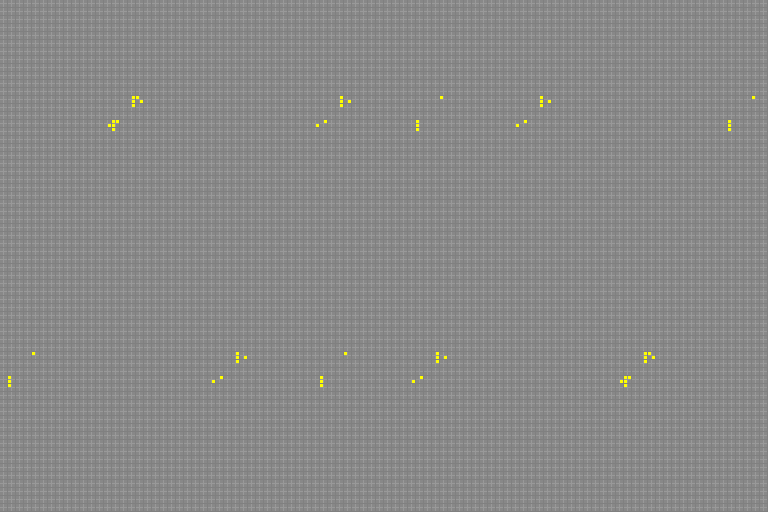
Similarly, the rule 0,2,1,3,8,10,9,11,4,6,5,7,12,14,13,15 or $1\leftrightarrow 2, 4\leftrightarrow 8$ sends all SE and NE cells at light speed to the west (summands with $T_{\W}$), and vice versa, again giving $p=1$ and period $M$.

Example 3

In the variant 0,1,2,3,8,9,10,11,4,5,6,7,12,13,14,15 or $1\leftrightarrow 2, 4\mapsto 4, 8\mapsto 8$, on the other hand, the gliders never go far: Now $p=2$ and the overall period remains 2 regardless of grid size, showing that any inductive argument exploiting the contraction maps $C_{2M,M}$ must start from a $2\times 2$-blocks grid as the base case, not from the single-block case! Spelling it out in the above formalism, there are terms with $T_{\W}$ and with $T_{\E}$, but the only products with matching projections in the second iterate end up with $T_{\W}T_{\E} = T_{\W}T_{\E} = T_0$ as the translation.

The second and third example do not depend on $M$ being a power of 2.

A final simplification

Fortunately, it turns out to be unnecessary to keep track of all the iterated $XPRPXRP$ business. Once we've computed the single iterate $A$, we can simply suppress all terms that contain vanishing matrix elements $PRP$, and all products where two different projection idempotents meet each other, and keep the surviving summands, with the mess hidden inside a black box: E.g., what the $k$-th iterate of the northwest-gliding summand does (if $P_{\NW}RP_{\SE}$ is nonzero) is fully captured by \begin{equation}P_{\SE}T_{\NW}^k\blacksquare P_{\SE}\,.\end{equation}

Example 4

Among the simplest nontrivial rules is 0,1,4,5,2,3,6,7,9,8,13,12,11,10,15,14 or $1\mapsto 1, 2\leftrightarrow 4, 8\mapsto 9$. The lit SW cells race NE and vice versa, independently of anything else, so I'll be omitting them from the following expressions. The NW and SE cells couple to each other; their contribution to the single iterate $A$ is: \begin{align} P_{\NW} (T_0) \blacksquare P_{\NW} & + \\ P_{\NW} (T_0) \blacksquare P_{\SE} & + \\ P_{\SE} (T_{\NW}) \blacksquare P_{\NW} & + \\ P_{\SE} (T_{\NW} + T_0) \blacksquare P_{\SE}\end{align}

Squaring this expression and collecting the translations gives: \begin{align} P_{\NW} (T_{\NW} + T_0) \blacksquare P_{\NW} & + \\ P_{\NW} (T_{\NW}) \blacksquare P_{\SE} & + \\ P_{\SE} (T_{\NW}^2) \blacksquare P_{\NW} & + \\ P_{\SE} (T_{\NW}^2 + T_{\NW} + T_0) \blacksquare P_{\SE}\end{align}

And the third iterate is: \begin{align} P_{\NW} (T_{\NW}^2 + T_{\NW} + T_0) \blacksquare P_{NW} & + \\ P_{\NW} (T_{\NW}^2 + T_0) \blacksquare P_{SE} & + \\ P_{\SE} (T_{\NW}^3 + T_{\NW}) \blacksquare P_{NW} & + \\ P_{\SE} (T_{\NW}^3 + T_{\NW}^2 + T_0) \blacksquare P_{\SE}\end{align}

Contracting this to a $1\times1$ grid by setting all translations equal to $T_0$, we get the identity map (NB also on the omitted SW and NE terms), thus $p=3$.

Contracting it to a $2\times 2$ grid amounts to setting the squares of all translations equal to $T_0$; the middle two terms vanish due to cancellation modulo 2, and we're left with the antipodal translation (again, also on the SW and NE terms which I've omitted): \begin{align} P_{\NW} (T_{\NW}) \blacksquare P_{\NW} & + \\ P_{\NW} (0) \blacksquare P_{\SE} & + \\ P_{\SE} (0) \blacksquare P_{\NW} & + \\ P_{\SE} (T_{\NW}) \blacksquare P_{\SE}\end{align} which is an involution on the space of grid states, confirming the overall period 6.

Lifting this inductively to $M\times M$ grids where $M$ is a power of 2 now reduces to a computation with binomial and multinomial coefficients modulo 2.

In general...

Further complications come from translation relations like $T_{\NW} = T_{\W}T_{\N}$.

We're left having to perform computations in $\mathbb{F}_2[T]$. The summands could be organized by paths in a Cayley graph of the group of translations $T$, with individual steps depending on the nonzero matrix elements of $R$, but I'm not sure whether that helps.

Afterthought:

We don't even need the black boxes! All these $P_{\NW} (T_{\NW}^2 + T_0) \blacksquare P_{\SE}$ (etc.) terms are bona fide matrix elements - and we need to keep only their $T_{\NW}^2 + T_0$ (etc.) parts when we arrange them into a $4\times 4$ matrix (which we may again call $A$) whose rows and columns are indexed by $\{\NW,\NE,\SW,\SE\}$. So we can work in a matrix algebra over the commutative algebra $\mathbb{F}_2[T]$, and in fact in the commutative matrix subalgebra generated by $A$.

But I still don't see how to extract from this a uniform inductive argument that would correctly predict the periods for all linear invertible rules on grids of power-of-two diameter.

Answer 4

So I have a proof of the low period phenomenon that works for all cellular automata prime characteristics $p$ and all finite dimensions (i.e. for linear cellular automata whose alphabet is a vector space of characteristic $p$ over a finite $p$-group). The general result can quite easily be verified empirically. These cellular automata could be applied to the reversible symmetric cryptosystems of the future since functions $f$ where $f^{m}=\textrm{Id}$ for some $m$ which are easily computable by a reversible computer will be important components of cryptographic hash functions of the future.

Let $G$ be a group and $A$ be a set. Then define $\phi_{g}:A^{G}\rightarrow A^{G}$ by letting $\phi_{g}(x_{h})_{h\in G}=(x_{g+h})_{h\in G}$. A cellular automaton over the group $G$ and the alphabet $A$ is a map $\tau:A^{G}\rightarrow A^{G}$ such that $\tau\phi_{g}=\phi_{g}\tau$ for all $g\in G$.

If $G$ is a group and $V$ is a vector space over a finite field $K$, then let $\textrm{LCA}(G;V)$ denote the collection of all linear cellular automata over the group $G$ with alphabet $V$. Let $c_{a}=(a)_{g\in G}\in V^{G}$ for each $a\in A$. If $V$ is a vector space over a field $K$ and $G$ is a group, the define a homomorphism $\Gamma:\textrm{LCA}(G;V)\rightarrow\textrm{End}_{K}(V)$ by letting $c_{\Gamma(\tau)(a)}=\tau(c_{a})$.

Theorem: Let $K$ be a finite field of prime characteristic $p$ and let $V$ be a vector space over $K$. Let $G=Z_{p^{a_{1}}}\times Z_{p^{a_{r}}}$. Let $m=p^{a_{1}}+...+p^{a_{r}}$. Let $n'$ be a natural number such that $p^{n'}\geq m$ and let $n=p^{n'}$.

1. Suppose that $r\in \textrm{LCA}(G;V)$ and $\Gamma(r)=0$. Then $r^{m}=0$.

2. Suppose that $r\in \textrm{LCA}(G;V)$ and $\Gamma(r)=1$. Then $r^{n}=1$.

3. Suppose that $r\in\textrm{LCA}(G;V)$ and $\Gamma(r)^{k}=0$. Then $r^{km}=0$.

4. Suppose that $r\in\textrm{LCA}(G;V)$ and $\Gamma(r)^{k}=1$. Then $r^{kn}=1$.

Proof: Statement 2 follows from statement 1; if $\Gamma(r)=1$, then $\Gamma(r-1)=0$, so $r^{n}-1=(r-1)^{n}=0$, hence $r^{n}=1$. Statements 2-4 therefore all follow from statement $1$, so it suffices to prove statement 1.

Suppose that $\Gamma(r)=0$. Now, suppose that $$r(x_{\alpha})_{\alpha\in G}=(\sum_{\beta\in G}R_{\beta}x_{\alpha+\beta})_{\alpha\in G}.$$ Then since $\Gamma(r)=0$, we know that $\sum_{\beta\in G}R_{\beta}=0$, so $$R_{0}=-\sum_{\beta\in G^{+}}R_{\beta}.$$ Therefore, $$r^{m}(x_{\alpha})_{\alpha\in G}=(\sum_{\beta_{1},...,\beta_{m}\in G^{+}}\sum_{u_{1},...,u_{m}\in\{0,1\}^{m}}(-1)^{m+u_{1}+...u_{m}}R_{\beta}x_{\alpha+u_{1}\beta_{1}+...u_{m}\beta_{m}})_{\alpha\in G}$$ $$=(\sum_{\beta_{1},...,\beta_{m}\in G^{+}}R_{\beta}\sum_{u_{1},...,u_{m}\in\{0,1\}^{m}}(-1)^{m+u_{1}+...u_{m}}x_{\alpha+u_{1}\beta_{1}+...u_{m}\beta_{m}})_{\alpha\in G}.$$

It therefore suffices to show that $$\sum_{u_{1},...,u_{m}\in\{0,1\}^{m}}(-1)^{m+u_{1}+...u_{m}}x_{\alpha+u_{1}\beta_{1}+...u_{m}\beta_{m}}=0$$ for all $\alpha,\beta_{1},...,\beta_{m}\in G$.

To verify this claim, we shall verify that $$\sum_{u_{1},...,u_{m}\in\{0,1\}^{m}}(-1)^{m+u_{1}+...u_{m}}\cdot(\alpha+u_{1}\beta_{1}+...u_{m}\beta_{m})=0$$ where the element $$(-1)^{m+u_{1}+...u_{m}}\cdot(\alpha+u_{1}\beta_{1}+...u_{m}\beta_{m})$$ is considered as an object in the group ring $K[G]$, Take note that $$\sum_{u_{1},...,u_{m}\in\{0,1\}^{m}}(-1)^{m+u_{1}+...u_{m}}\cdot(\alpha+u_{1}\beta_{1}+...u_{m}\beta_{m})=\alpha\cdot(\beta_{1}-1)\cdot...\cdot(\beta_{m}-1).$$

Now, take note that the group-ring $K[G]$ is isomorphic to the ring $$K[x_{1},...,x_{r}]/\langle x_{1}^{p^{a_{1}}}-1,...,x_{r}^{p^{a_{r}}}-1\rangle,$$ and by this isomorphism, $\alpha\cdot(\beta_{1}-1)\cdot...\cdot(\beta_{m}-1)$ is sent to $$\mathbf{x}^{\alpha}\cdot(\mathbf{x}^{\beta_{1}}-1)\dots(\mathbf{x}^{\beta_{m}}-1)+\langle x_{1}^{p^{a_{1}}}-1,...,x_{r}^{p^{a_{r}}}-1\rangle.$$ Now, $$K[x_{1},...,x_{r}]/\langle x_{1}^{p^{a_{1}}}-1,...,x_{r}^{p^{a_{r}}}-1\rangle= K[x_{1},...,x_{r}]/\langle (x_{1}-1)^{p^{a_{1}}},...,(x_{r}-1)^{p^{a_{r}}}\rangle$$ and the automorphism $\Phi:K[x_{1},...,x_{r}]\rightarrow K[x_{1},...,x_{r}]$ defined by $\Phi(x_{i})=x_{i}+1$ induces an isomorphism on the quotient rings $$\Phi^{*}:K[x_{1},...,x_{r}]/\langle x_{1}^{p^{a_{1}}}-1,...,x_{r}^{p^{a_{r}}}-1\rangle \rightarrow K[x_{1},...,x_{r}]/\langle x_{1}^{p^{a_{1}}},...,x_{r}^{p^{a_{r}}}\rangle$$ and $$\Phi^{*}(\mathbf{x}^{\alpha}\cdot(\mathbf{x}^{\beta_{1}}-1)\dots(\mathbf{x}^{\beta_{m}}-1)+\langle x_{1}^{p^{a_{1}}}-1,...,x_{r}^{p^{a_{r}}}-1\rangle)$$ $$=p(\mathbf{x})f_{1}(\mathbf{x})\dots f_{m}(\mathbf{x})+\langle x_{1}^{p_{a_{1}}},\dots,x_{r}^{p_{a_{r}}}\rangle$$ for some polynomials $f_{1},...,f_{m}$ with $f_{1}(\mathbf{0})=\dots=f_{m}(\mathbf{0})=0$. Since $$f_{1}(\mathbf{0})=\dots=f_{m}(\mathbf{0})=0,$$ we conclude that $f_{i}=\sum_{\beta\neq 0}a_{i,\beta}\mathbf{x}^{\beta}$. However, $$f_{1}(\mathbf{x})\dots f_{m}(\mathbf{x})=\sum_{\beta_{1}\neq 0,...,\beta_{m}\neq 0}a_{1,\beta_{1}}...a_{m,\beta_{m}}\mathbf{x}^{\beta_{1}+...+\beta_{m}}\in \langle x_{1}^{p_{a_{1}}},\dots,x_{r}^{p_{a_{r}}}\rangle.$$ Therefore, $$p(\mathbf{x})f_{1}(\mathbf{x})\dots f_{m}(\mathbf{x})+\langle x_{1}^{p_{a_{1}}},\dots,x_{r}^{p_{a_{r}}}\rangle=0.$$ We therefore conclude that $r^{m}(x_{\alpha})_{\alpha\in G}=0$. $\mathbf{QED}$