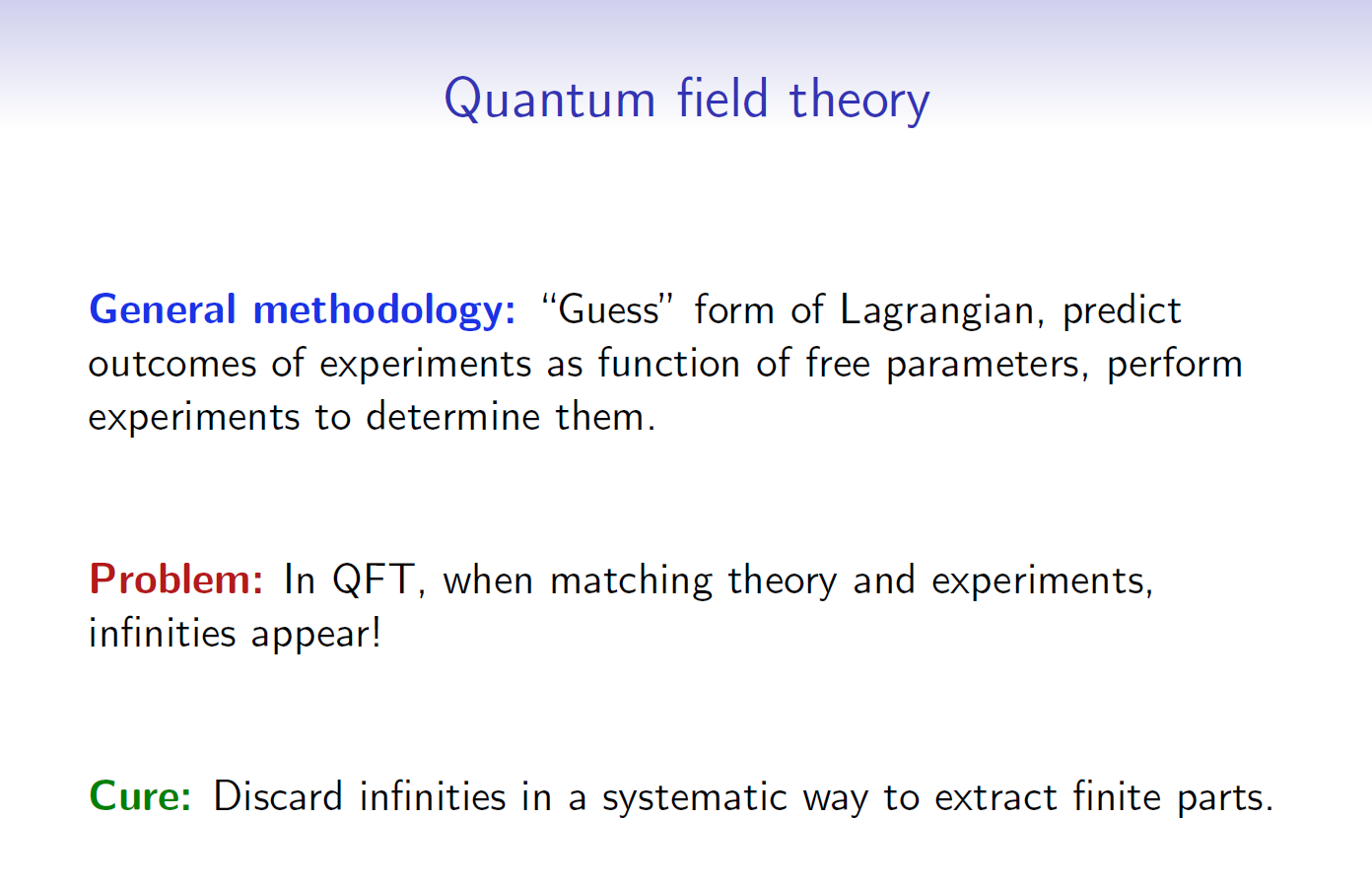
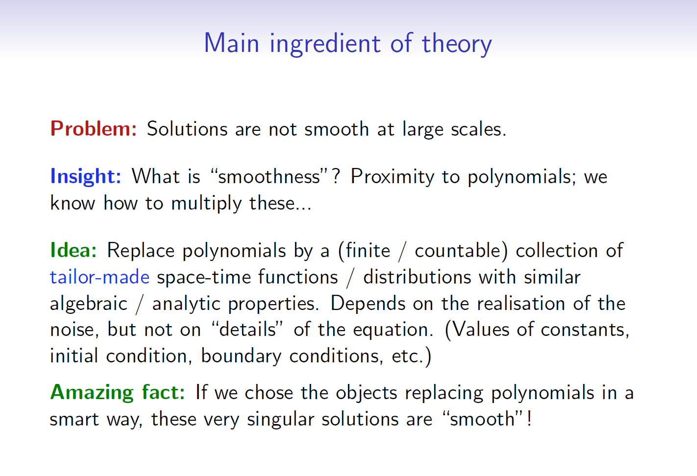
Let me comment on points 4) and 5). The problem with infinities in QFT or traditional equilibrium statistical field theory
is related to the one addressed by Martin's theory but there are some differences. For concreteness let me talk about the $\phi^4$ model
only. Mathematically, the problem it poses is to make sense of the probability measure
$$
\frac{1}{\mathcal{Z}}\exp\left(
-\int_{\mathbb{R}^d}\{
\frac{1}{2} (\nabla\phi)^2(x)+\mu \phi(x)^2+g\phi(x)^{4}
\} d^dx
\right)\ D\phi
$$
on the "space of all functions" $\phi:\mathbb{R}^d\rightarrow\mathbb{R}$. This is the kind of heuristic formulas
one finds in physics QFT textbooks. The symbol $D\phi$ stands for Lebesgue measure on this space of functions
and $\mathcal{Z}$ is a normalization constant so the full space has measure one as befits a probability measure.
Now let's turn this into a well posed mathematical question.
First remove the $\phi^2$ and $\phi^4$ terms, i.e., consider the case $\mu=g=0$. Then this measure $\mu_{C_{-\infty}}$
makes perfect sense. It is the centered Gaussian measure on the space of temperate distributions $S'(\mathbb{R}^d)$
and with covariance $C_{-\infty}$ given by
$$
C_{-\infty}(f,g)=\frac{1}{(2\pi)^{d}}\int_{\mathbb{R}^d}\frac{\overline{\widehat{f}(\xi)}
\widehat{g}(\xi)}{|\xi|^{2}} d^d\xi
$$
for all test functions $f$ and $g$ in $S(\mathbb{R}^d)$. Using this first rigorous step, one can reformulate
the problem as that of making sense of
$$
\frac{1}{\mathcal{Z}}\exp\left(
-\int_{\mathbb{R}^d}\{
\alpha (\nabla\phi)^2(x)+\mu \phi(x)^2+g\phi(x)^{4}
\} d^dx
\right)\ d\mu_{C_{-\infty}}(\phi)
$$
with a new normalization constant $\mathcal{Z}$ that I will still keep calling $\mathcal{Z}$.
I also introduced the "wave function renormalization coupling constant" $\alpha$ for more generality.
We made a bit of progress (we avoided the problematic Lebesgue measure $D\phi$),
but this still does not make mathematical sense because $\mu_{C_{-\infty}}$ is supported on nasty Schwartz distributions
and pointwise powers like $\phi^2$ and $\phi^4$ are ill-defined, just like $\Phi^3$ in Martin's answer. This is the source
of the UV (ultraviolet) infinities. There are also IR (infrared) problems due to the integration inside the exponential
being over $\mathbb{R}^d$ instead of a compact set. To address these issues, we need what the French call troncature et
régularisation. Let $\rho_{\rm UV}$ be a mollifier, i.e., a compactly supported $C^{\infty}$ function
$\mathbb{R}^d\rightarrow\mathbb{R}$ with $\int \rho_{\rm UV}=1$.
Let $\rho_{\rm IR}$ be a cut-off function, i.e., a nonnegative compactly supported $C^{\infty}$ function
$\mathbb{R}^d\rightarrow\mathbb{R}$ which is equal to 1 in a neighborhood of the origin. To slice Fourier momenta
into (Littlewood-Paley) shells we introduce an integer $L>1$, not necessarily equal to 2 as is customary in
harmonic analysis. For $r,s\in\mathbb{Z}$, define the rescaled functions $\rho_{{\rm UV},r}(x)=L^{-dr}\rho_{\rm UV}(L^{-r}x)$
and $\rho_{{\rm IR},s}(x)=\rho_{\rm IR}(L^{-s}x)$, and consider the probability measure $\nu_{r,s}$ given by
$$
\frac{1}{\mathcal{Z}}\exp\left(
-\int_{\mathbb{R}^d}\rho_{{\rm IR},s}(x)\{
\alpha (\nabla\phi)^2(x)+\mu \phi(x)^2+g\phi(x)^{4}
\} d^dx
\right)\ d\mu_{C_{r}}(\phi)
$$
where $\mu_{C_r}$, or regularized Gaussian measure, is the direct image of $\mu_{C_{-\infty}}$
by the convolution map $\phi\mapsto \rho_{{\rm UV},r}\ast\phi$.
In other words, $\mu_{C_r}$ is the centered Gaussian measure with covariance
$$
C_{r}(f,g)=\frac{1}{(2\pi)^{d}}\int_{\mathbb{R}^d}\frac{|\widehat{\rho_{{\rm UV},r}}(\xi)|^2\ \overline{\widehat{f}(\xi)}
\widehat{g}(\xi)}{|\xi|^{2}} d^d\xi\ .
$$
A good metaphor would be to say that your orginal flat-screen TV was too smart. The linear size of the
screen was $L^s=\infty$ and that of a pixel was $L^r=0$. Instead one should make $r$ and $s$ finite so that $\nu_{r,s}$
is mathematically well defined, and then study the limit where $r\rightarrow-\infty$ and $s\rightarrow\infty$
in the sense of
weak convergence of probability measures on the topological space $S'(\mathbb{R}^d)$.
Now renormalization theory in physics tells us that unless we allow the couplings $(\alpha,\mu,g)$ to depend on the
UV cut-off scale $r$, the following is more likely to happen: 1) we don't converge (e.g., loss of tightness), 2)
we converge to something utterly uninteresting like the atomic measure on the singleton $\{\phi=0\}$, 3) we
converge to something less trivial but still uninteresting, namely, a Gaussian measure like the GFF $\mu_{C_{-\infty}}$
or white noise, or massive free fields interpolating between the two.
Therefore the weak limit we need to study depends on the choice of bare ansatz $(\alpha_r,\mu_r,g_r)_{r\in\mathbb{Z}}$
(or rather the germ of this sequence at $r=-\infty$). Finally, the well posed mathematical question I promised,
regarding trying to make sense of the original $\phi^4$ functional integral is the following.
Problem: Find an explicit parametrization of all weak limits (of probability measures on $S'(\mathbb{R}^d)$)
given by $\lim_{r\rightarrow-\infty}\lim_{s\rightarrow\infty}\nu_{r,s}$ for all possible choices of bare ansatz
$(\alpha_r,\mu_r,g_r)_{r\in\mathbb{Z}}$.
What renormalization theory in physics also tells us is that although it seems one has a hugely infinite-dimensional
amount of freedom in choosing the sequence $(\alpha_r,\mu_r,g_r)_{r\in\mathbb{Z}}$, the set $\mathscr{T}$
of weak limit points
is a finite-dimensional variety. For $d=3$, one expects three parameters or "renormalized coupling constants"
$(\alpha_{\rm R},\mu_{\rm R},g_{\rm R})$ suffice.
One can even get rid of $\alpha_{\rm R}$ if one quotients by taking constant
multiples of the random field $\phi$.
There are rigorous renormalization group techniques for constructing portions of $\mathscr{T}$. Kupiainen's work mentioned
by Ofer is an adaptation of these techniques to the time-dependent rough SPDE setting.
The above is what I call the non-anchored Gibbsian way
of trying to construct elements $\nu\in\mathscr{T}$. There is a completely different approach which I call the
anchored stochastic quantization approach. There one need to make sense of the SPDE in Martin's answer, which he
did locally in time. Then one needs to understand this SPDE globally in time and construct an invariant
measure which gives $\nu\in\mathscr{T}$. This is also fraught with difficulties but there has been quite a bit of progress in this direction
(see, e.g., this article related to invariant measures and Martin's comment below).
The key difference between the two approches is that in the non-anchored setting one does not have a fixed probability space
to work with. In the second anchored situation one does since all fields are functionals of the driving noise. In the anchored setting,
$L^2$ estimates involving second moments only are enough to prove convergence in probability and thus in
law for the random fields of interest. In the non-anchored situation one needs to control all moments
(correlation functions) with uniform $n!$ bounds on these moments.
It is hard to say more as an MO answer, but you can see these papers for further explanations:
- "A second-quantized Kolmogorov-Chentsov theorem via the operator product expansion", published here.
- "Towards three-dimensional conformal probability", published here.
- "QFT, RG, and all that, for mathematicians, in eleven pages"
Before reading these articles it may helpful to consult the slides of my recent Colloquium talk "A Toy Model for Three-Dimensional Conformal Probability". They should be much easier to follow since they contain lots of pictures.
The article in bullet point 1) provides an alternate way of defining pointwise products of random distributions
(like $\phi^2$ and $\phi^4$ above) using Wilson's operator product expansion (OPE). Regarding 5) in the OP's question,
I believe it would be of great interest to prove that the moments of the solution $\Phi$ constructed by Martin
satisfy the (dynamical version) of Wilson's OPE, and then compare $\Phi^3$ obtained by the theory of regularity structures
with the one constructed (from the OPE) in my 2nd quantized KC paper.
Update (Jan 27, 2018): The article by Mourrat and Weber mentioned by Martin in his comment below has now appeared in CMP, see here. It provides a new construction of the scalar $\phi^4$ model in three dimensions, in finite volume.
Update (Jan 21, 2019): Progress in the area has been quite fast and, since my last update, the limitation to finite volume has been overcome as mentioned in Martin's comment below. For the infinite volume treatment of $\phi_3^4$ via the stochastic quantization method see this article by Gubinelli and Hofmanová (with the paracontrolled approach) and the one by Moinat and Weber mentioned below (with the regularity structures approach).


