What explains the asymptotic and the pattern in this sequence related to Riemann zeta zeros?

Question

As the starting point for my experiment I assumed that the imaginary parts of the Riemann zeta zeros are of the form:

$$\Im \{ \rho_n \} = \frac{2\pi}{\log x_n}$$

where $x_n$ is unknown. Therefore I solved for $x_n$ and got this integer sequence:

$$\Large a_1(n) = (n+1) \left(\left[\frac{1}{e^{\frac{2 \pi }{\Im(\rho _{n+1})}}-1}\right]-\left[\frac{1}{e^{\frac{2 \pi }{\Im(\rho _n)}}-1}\right]\right)$$

where $\left[ \text{number}\right]$ is the round or nearest integer function. This is a sequence starting:

$a_1 =\;$2, 3, 0, 5, 0, 7, 0, 9, 0, 11, 0, 13, 0, 15, 0, 17, 0, 19, 0, 0, 22, 0, 0, 25, 0, ... $ \; a_1(n)$

I then deleted the zeros in that sequence to get:

$a_2 =\;$2, 3, 5, 7, 9, 11, 13, 15, 17, 19, 22, 25, 27, 30, 33, 36, 39, 42, 45, 48, 51, 54, 57, 61, 64,...

Now a search in The On-Line Encyclopedia of Integer Sequences (OEIS) suggests that the first few terms are sequence A092919. Therefore the sequence:

$$b(k)=\sum _{n=1}^{k+2} \text{Round}[\log (n)]$$ where $k$ is a natural number: $$k=1,2,3,4,5,...$$

agrees with the beginning of $a_2 \;$.

$b = \;$ 2, 3, 5, 7, 9, 11, 13, 15, 17, 19, 22, 25, 28, 31,...

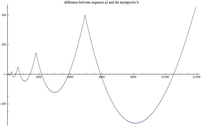
With Odlyzko's list of the 100000 first Riemann zeta zeros I plotted the difference $a_2 - b$: .
.
.

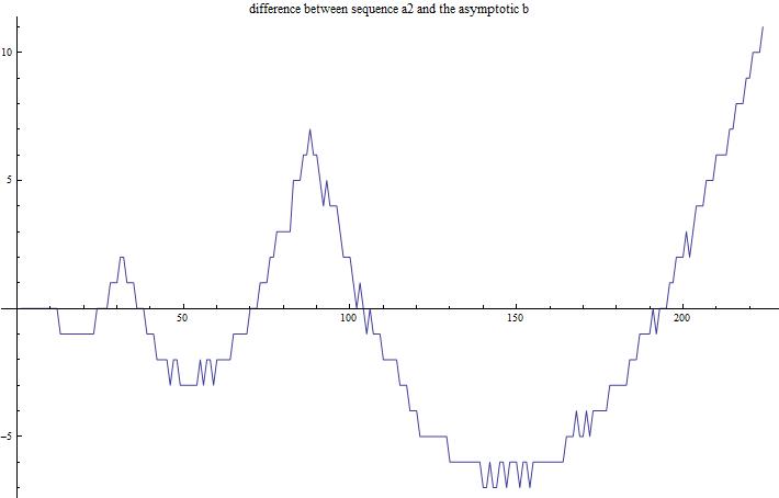
The smoothness is only apparent at a such zoomed out plot. Actually when zooming in at the beginning it looks like this:

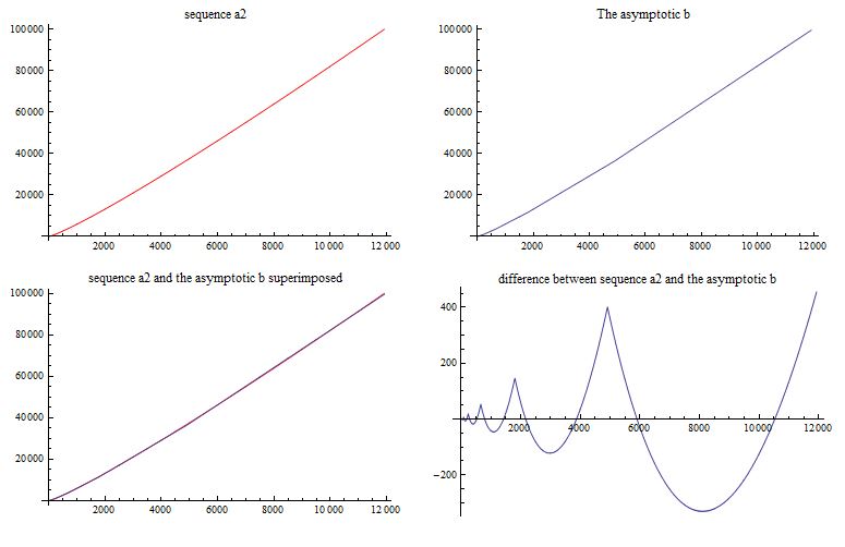
Just for clarity I plotted the sequence $a_2$ and its conjectured asymptotic $b$ separately also:

Mathematica 8 code for the plots:

(*start*)
(*Mathematica 8*)
nn = 1000;
Monitor[a1 = 
  Table[(n + 1)*(Round[(Exp[1/(Im[ZetaZero[n + 1]]/(2*Pi))] - 1)^-1] -
       Round[(Exp[1/(Im[ZetaZero[n]]/(2*Pi))] - 1)^-1]), {n, 1, 
    nn}], n]
a2 = DeleteCases[a1, 0]
b = Table[Sum[Round[Log[n]], {n, 1, k}], {k, 3, Length[a2] + 2}]
cc = a2 - b;
cc[[1 ;; 20]]
Label
g1 = ListLinePlot[a2, PlotStyle -> Red, PlotLabel -> "sequence a2"]
g2 = ListLinePlot[b, PlotLabel -> "asymptotic b"]
g3 = Show[g1, g2, 
  PlotLabel -> "sequence a2 and asymptotic b superimposed"]
g4 = ListLinePlot[cc, 
  PlotLabel -> "difference between sequence a2 and asymptotic b"]
GraphicsGrid[{{g1, g2}, {g3, g4}}]
(*end*)

Is the sequence $b$ asymptotic to sequence $a_2$ and what explains the large scale repeating pattern in the difference $a_2 - b$?

Answer 1

This has almost nothing to do with the zeros of zeta. To show it you can substitute $\frac{\Im(\rho_n)}{2\pi}$ in your program with an adequate approximation.

Since the number of zeros of zeta $$N(T)\approx\frac{T}{2\pi}\log \frac{T}{2\pi}-\frac{T}{2\pi}$$ a good approximation to $\frac{\Im(\rho_n)}{2\pi}$ is the solution of the equation $$n= x\log x-x$$ the solution is near $x_0=n/\log n$.

I used

f[1]=1; f[2]=2; f[n_] := Module[{x}, x /. FindRoot[n == x Log[x] - x, {x, n/Log[n]}][[1]]];

instead of $\frac{\Im(\rho_n)}{2\pi}$ and we obtained very similar plots. With the same large scale repeating pattern in the difference $a_2-b$.