21
$\begingroup$

Let $S^{d-1} = \{x \in \mathbb R^d: \|x\| = 1\}$ denote the unit sphere in $\mathbb R^d$. Let $v$, $w$ be drawn uniformly at random from $S^{d-1}$, conditioned on their inner product being equal to $\langle v, w \rangle = \cos \theta$. In other words, $v$ and $w$ have a fixed common angle $\theta$. I am interested in the probability that these two vectors lie in the same orthant, say the all-positive orthant, averaged over all possible $v$ and $w$: $$f_d(\theta) = \Pr(v > 0 \mid w > 0, \ \langle v, w \rangle = \cos \theta).$$ Here $v > 0$ means that all $d$ coordinates of $v$ are positive.

In particular, I am interested in the asymptotics of large $d \to \infty$ of $f_d(\theta)$ for $\theta \in (0, \frac{1}{2} \pi)$. Equivalently, as $f_d$ scales exponentially in $d$, I'm interested in the function $$g(\theta) = \lim_{d \to \infty} f_d(\theta)^{1/d}.$$

Note that an approximation to the above probabilities can be obtained by replacing the uniform distribution over the sphere by a multivariate Gaussian distribution, where each coordinate is independently drawn from a Gaussian $\mathcal{N}(0, \frac{1}{d})$. For large $d$, with overwhelming probability such a random vector will have norm $1 \pm o(1)$, and with overwhelming probability two such random vectors will have inner product $o(1)$. If we ignore the fact that the norms of such vectors may not exactly be equal to $1$ and that two random vectors may not be exactly orthogonal (which is why this is only an approximation), then two vectors $v$ and $w$ from the sphere with angle $\theta$ can be generated by taking $v = n_1$ and $w = (\cos \theta) n_1 + (\sin \theta) n_2$ for two independent random Gaussian vectors $n_1, n_2 \sim \mathcal{N}(0, \frac{1}{d})^d$. These lie on the sphere exactly if $n_1, n_2$ have norm $1$, and their angle is then equal to $\theta$ if and only if $n_1$ and $n_2$ are orthogonal.

With this approximation, probabilities can be computed quite easily, as different coordinates are independent and probabilities multiply. However, I'm looking for more precise estimates than using this Gaussian approximation of the uniform distribution on the sphere.

So far I've tried sharing this problem with a few others in the department, and rewriting the probability to computing the expected volume of the intersection of the sphere with $d$ orthogonal hyperplanes, but so far nothing led anywhere. Any pointers on how to solve this would be greatly appreciated!


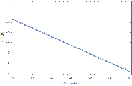
Update: To verify/compare different approaches, simulations for $\theta = \arccos 0.9$ in dimensions $d \in \{10, \dots, 40\}$ show the following trends for $\ln f$:

enter image description here

The points are the simulation results (using 100.000-500.000 experiments each, so that the number of successes was at least a few hundred) and the line is the linear fit $-0.0133857 - 0.170074 d$, or equivalently $f(\arccos 0.9) \approx C \cdot 0.8436^d$ for a constant $C \approx 1$. This suggests that $g(\arccos 0.9) \approx 0.8436$. The answers given so far say:

  • Carlo's answer: $0.66$
  • Other answer (main): $1.08$
  • Other answer (alternative): $0.71$

So perhaps all answers so far are still far off when $\theta$ is small and the inner product between $v$ and $w$ is large.

$\endgroup$
20
  • $\begingroup$ I would have guessed that the gaussian approximation is quite accurate. Are you sure it isn't? $\endgroup$ Commented Nov 14, 2015 at 3:20
  • 1
    $\begingroup$ Follow up on my earlier comment: in fact, you are asking about large deviations for quadratic forms, as follows: by Bayes', you are considering, with $A=\sum \eta_i g_i/\sqrt{\sum g_i^2 \sum \eta_i^2}$, the expression $$P(g_i>0,\eta_i>0,A\sim cos \theta)/P(g_i>0, A\sim \cos \theta).$$ Here, $g_i$ and $\eta_i$ are iid N(0,1).Computing the exponential rate of decay of both numerator and denominator then becomes a (tedious, but solvable) question on LDP for quadratic forms in i.i.d. random variables. I don't have time right now to fill in the details, hopefully someone else can follow up on that. $\endgroup$ Commented Nov 17, 2015 at 20:54
  • 1
    $\begingroup$ @TMM, I'm not sure they are different problems. If $A$ is the event of having angle in $[\theta-\epsilon,\theta+\epsilon]$ and $B$ is the event of both being in the positive orthant, then Bayes' Thm says that $P(A|B)/P(B|A)=P(A)/P(B)$. Since $P(A)$ and $P(B)$ are easy, you can find $P(B|A)$ if you can find $P(A|B)$. Conditioning iid normals on being in the positive orthant is the same as using iid $|N(0,1)|$s, isn't it? $\endgroup$ Commented Nov 18, 2015 at 13:47
  • 1
    $\begingroup$ I think my comment above and standard LD is all you need. Let me expand a bit. You are welcomed to contact me by email if needed. Let's say you want to compute (see my comment above) $P(\eta_i>0,g_i>0, B)=P(B|\eta_i>0,g_i>0) 2^{-2n}$ where $B=\{|A-\cos \theta|<\epsilon\}$. Rewrite the conditional probability on the right as $Q(B)$, note that under $Q$ the $\eta$'s, $g$'s are still iid. Now on exponential scale, you have that $Q(B)\sim \max_{y,z} Q(\sum \eta_i g_i\sim y N,\sum \eta_i^2\sim z^2N,\sum g_i^2\sim y^2/ z^2 \cos(\theta)^2$ $\endgroup$ Commented Feb 4, 2017 at 4:53
  • 1
    $\begingroup$ Now the latter probability is computed by the Gartner-Ellis theorem in $R^3$: the exponential rate is $I(y,z^2,y^2/z^2\cos(\theta)^2)$ where $I$ is the Legendre transform of $\Lambda(\theta_1,\theta_2,\theta_3)=\log E_Q(e^{\theta_1 \eta_1 g_1}\cdot e^{\theta_2 \eta_1^2} \cdot e^{\theta_3 g_1^2})$. This computation is an explicit, if tedious, two dimensional integral. One can numerically compute $\Lambda$, its Legendre transform, and then optimize over $z,y$ as stated. For notation etc see my book with Dembo, in the section on Gartner-Ellis theorem. $\endgroup$ Commented Feb 4, 2017 at 4:55

3 Answers 3

5
+100
$\begingroup$

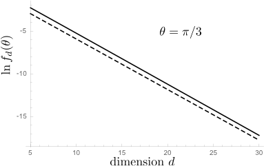
So I made this Gaussian approximation and find for $\theta=\pi/3$ a $d$-dependence of $f_d(\theta)$ that is well described by

$$f_d(\pi/3)\approx 2^{-d}e^{d/\pi^2}\Rightarrow g(\pi/3)\approx\tfrac{1}{2}e^{1/\pi^2}=0.553\;\;\;(1)$$

The plot shows the result of the Gaussian approximation (solid curve) and the asymptotic form (1) (dashed curve) on a log-normal scale, with a slope that matches quite well.

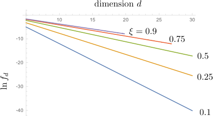
And here is the Gaussian approximation for several values of $\xi=\cos\theta$:

From the slope I estimate that

$$g(\theta)=\begin{cases} 0.66&\text{for}\;\cos\theta=0.9\\ 0.63&\text{for}\;\cos\theta=0.75\\ 0.55&\text{for}\;\cos\theta=0.5\\ 0.41&\text{for}\;\cos\theta=0.25\\ 0.25&\text{for}\;\cos\theta=0.1 \end{cases} $$


Gaussian approximation

Denoting $\xi=\cos\theta$ we seek the probability

$$f_d(\xi)=2^d \frac{X_d(\xi)}{Y_d(\xi)},$$

as a ratio of the two expressions \begin{align} &X_d(\xi)=\int d\vec{x}\int d\vec{y}\, \exp(-\tfrac{d}{2}\Sigma_n x_n^2) \exp(-\tfrac{d}{2}\Sigma_n y_n^2)\delta\left(\xi-\Sigma_n x_n y_n\right)\prod_{n=1}^d \Theta(x_n)\Theta(y_n),\\ &Y_d(\xi)=\int d\vec{x}\int d\vec{y}\, \exp(-\tfrac{d}{2}\Sigma_n x_n^2) \exp(-\tfrac{d}{2}\Sigma_n y_n^2)\delta\left(\xi-\Sigma_n x_n y_n\right) . \end{align} (The function $\Theta(x)$ is the unit step function.) Fourier transformation with respect to $\xi$, \begin{align} \hat{X}_d(\gamma)&= \int_{-\infty}^\infty d\xi\, e^{i\xi\gamma}X(\xi)\nonumber\\ &=\left[\int_{0}^\infty dx\int_{0}^\infty dy\,\exp\left(-\tfrac{d}{2}x^2-\tfrac{d}{2}y^2+ixy\gamma\right)\right]^d\nonumber\\ &=(d^2+\gamma^2)^{-d/2}\left(\frac{\pi}{2}+i\,\text{arsinh}\,\frac{\gamma}{d}\right)^d,\\ \hat{Y}_d(\gamma)&=\int_{-\infty}^\infty d\xi\, e^{i\xi\gamma}X(\xi)\nonumber\\ &=\left[\int_{-\infty}^\infty dx\int_{-\infty}^\infty dy\,\exp\left(-\tfrac{d}{2}x^2-\tfrac{d}{2}y^2+ixy\gamma\right)\right]^d\nonumber\\ &=(2\pi)^d(d^2+\gamma^2)^{-d/2}. \end{align} Inverse Fourier transformation gives for $\xi=1/2$ the solid line in the plot. The integrals are still rather cumbersome, so I have not obtained an exact expression for $g(\theta)$, but equation (1) shown as a dashed line seems to have pretty much the same slope.


Addendum (December 2015)

The answer of TMM raises the question, "how can the Gaussian approximation produce two different results"? Let me try to address this question here. To be precise, with "Gaussian approximation" I mean the approximation that replaces the individual components of the random $d$-dimensional unit vectors $v$ and $w$ by i.i.d. Gaussian variables with zero mean and variance $1/d$. It seems like a well-defined procedure, that should lead to a unique result for $g(\theta)$, and the question is why it apparently does not.

The issue I think is the following: The (second) calculation of TMM makes one additional approximation, beyond the Gaussian approximation for $v$ and $w$, which is that their inner product $v\cdot w$ has a Gaussian distribution, $$P(v \cdot w = \alpha | v, w > 0) \propto \exp\left(-\frac{d (\alpha \pi - 2)^2}{2 \pi^2 - 8}\right).\qquad[*]$$ The justification would be that this additional approximation becomes exact for $d\gg 1$, by the central-limit-theorem, but I do not think this applies, for the following reason: The approximation [*] breaks down in the tails of the distribution, when $|\alpha-2/\pi|\gg 1/\sqrt d$. So in the large-$d$ limit it only applies when $\alpha\rightarrow 2/\pi$, but in particular not for $\alpha\ll 1$.

$\endgroup$
7
  • $\begingroup$ $f$ above is already conditioned on $w > 0$ so I suppose your result would then be that $f \sim 2^{-d} e^{-d/\pi^2} \approx (0.553)^d$. That sounds about right, judging from experimental data; thanks! If you could work out the details for general $\theta \in (0, \frac{1}{2} \pi)$ that would be great, but I understand is that's too much to ask. $\endgroup$
    – TMM
    Commented Nov 18, 2015 at 0:35
  • $\begingroup$ clear enough, thanks! I have corrected for the conditioning on $w>0$ and added results for the Gaussian approximation for other values of $\theta$. $\endgroup$ Commented Nov 18, 2015 at 11:32
  • $\begingroup$ Thanks for the updates! One last question: could you provide a bit more information on how you generated those curves and estimated the slope? Did you also use the Gaussian approximation for that, with different $\xi$? I would like to get (approximations of) some more values of $g(\theta)$ but I'm not sure how to compute those numbers from the given expressions, even with mathematical software. $\endgroup$
    – TMM
    Commented Nov 19, 2015 at 14:02
  • $\begingroup$ Here are the lines of Mathematica code that generate the plot (in Gaussian approximation) for a chosen value of $\xi$; I just fitted a straight line to get the slope: numerator[d_,gamma_]:=(d^2 + gamma^2)^(-d/2) * (Pi/2 + I * ArcSinh[gamma/d])^d; denominator[d_,gamma_]:=(d^2 + gamma^2)^(-d/2) * (2 * Pi)^d; xi=1/2; Plot[Log[2^d*Re[NIntegrate[Exp[-I * xi * gamma] * numerator[d,gamma],{gamma,-Infinity, Infinity}]]/NIntegrate[Exp[-I * xi * gamma] * denominator[d,gamma],{gamma,-Infinity,Infinity}]], {d,5,30}] $\endgroup$ Commented Nov 19, 2015 at 14:34
  • $\begingroup$ Just a note: I've removed the "accepted"-mark as I'm not convinced anymore that this is the correct answer. See below for a different approach leading to a different answer. It is still a very useful and interesting answer showing an approach I had not considered, but it may not solve the problem. $\endgroup$
    – TMM
    Commented Dec 3, 2015 at 16:27
3
$\begingroup$

Thanks to Ofer Zeitouni, unless I made some serious mistakes somewhere in the calculations, I've been able to find the exact answer using large deviations theory. The derivation of the final result is a rather tedious affair, so I will just state the result here. Below $\mathcal{S}^{d-1}$ denotes (the uniform distribution over) the unit ball in $\mathbb{R}^d$. The proof can be found in the appendix here and is about 5 pages long.


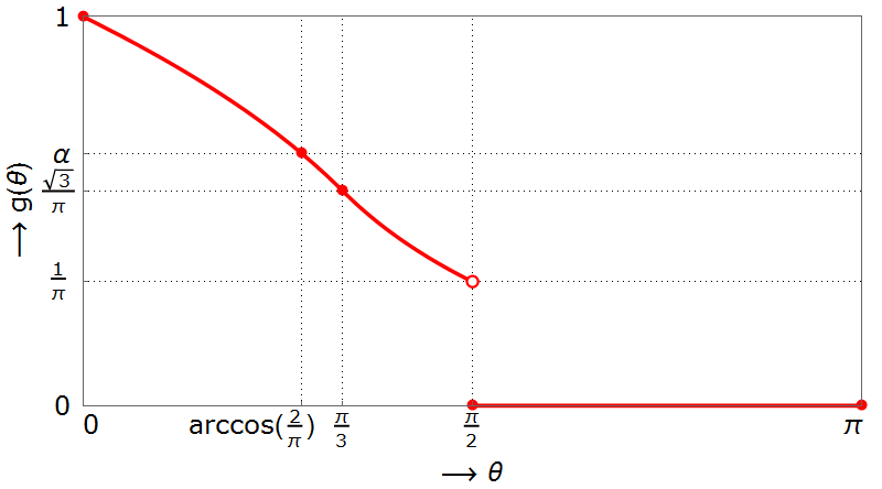
Theorem: Let $\mathbf{X}, \mathbf{Y} \sim \mathcal{S}^{d-1}$, let $\phi(\mathbf{X}, \mathbf{Y})$ denote the angle between $\mathbf{X}$ and $\mathbf{Y}$, and let \begin{align} f_d(\theta) = \mathbb{P}(\mathbf{X} > 0 \ | \ \mathbf{Y} > 0, \ \phi(\mathbf{X}, \mathbf{Y}) = \theta). \end{align} For $\theta \in (0, \arccos \frac{2}{\pi})$ (respectively $\theta \in (\arccos \frac{2}{\pi}, \frac{\pi}{3})$), let $\beta_0 \in (1, \infty)$ (respectively $\beta_1 \in (1, \infty)$) be the unique solution to: \begin{align} \arccos\left(\frac{-1}{\beta_0}\right) = \frac{(\beta_0 - \cos \theta) \sqrt{\beta_0^2 - 1}}{\beta_0 (\beta_0 \cos \theta - 1)} \, , \qquad \arccos\left(\frac{1}{\beta_1}\right) = \frac{(\beta_1 + \cos \theta) \sqrt{\beta_1^2-1}}{\beta_1 (\beta_1 \cos \theta + 1)} \, . \label{eq:beta} \end{align} Then, for large $d$, \begin{align} f_d(\theta) = \begin{cases} \left(\displaystyle\frac{(\beta_0 - \cos \theta)^2 }{\pi \beta_0 (\beta_0 \cos \theta - 1) \sin \theta}\right)^{d + o(d)}, & \qquad \text{if } \theta \in [0, \arccos \tfrac{2}{\pi}]; \\[3ex] \left(\displaystyle\frac{(\beta_1 + \cos \theta)^2}{\pi \beta_1 (\beta_1 \cos \theta + 1) \sin \theta}\right)^{d + o(d)}, & \qquad \text{if } \theta \in [\arccos \tfrac{2}{\pi}, \tfrac{\pi}{3}]; \\[3ex] \left(\displaystyle\frac{1 + \cos \theta}{\pi \sin \theta}\right)^{d + o(d)}, & \qquad \text{if } \theta \in [\tfrac{\pi}{3}, \tfrac{\pi}{2}); \\[3ex] 0, & \qquad \text{if } \theta \in [\tfrac{\pi}{2}, \pi]. \end{cases} \end{align}


To illustrate, the following figure shows $g(\theta) = \lim_{d\to \infty} f_d(\theta)^{1/d}$ against $\theta$. The constant $\alpha$ on the y-axis is $\alpha = \pi / (2 \sqrt{\pi^2 - 4}) \approx 0.648$. The dashed lines indicate the boundaries of the piece-wise parts in the theorem.

enter image description here

As stated in the OP, experiments suggested that $g(\arccos 0.9) \approx 0.8436$, and indeed from this theorem we find $g(\arccos 0.9)$ to be approximately $0.843$. This is quite different from Carlo's approximate solution based on Gaussians - if $\theta$ is close to $0$, the Gaussian approximation seems to be further off.

For the case $\theta = \frac{\pi}{3}$, the exact solution is $g(\frac{\pi}{3}) = \frac{\sqrt{3}}{\pi} \approx 0.5513$. Other answers based on different approximations all suggested $g(\frac{\pi}{3}) \in [0.55, 0.57]$ so here the Gaussian approximations are pretty accurate.

And as $\theta$ approaches $\frac{\pi}{2}$ from below, we curiously get $g(\theta) \to \frac{1}{\pi}$. In other words, two almost-orthogonal vectors in high dimensions are in the same orthant with probability proportional to $(\frac{1}{\pi})^{d + o(d)}$. I'm not sure if there is a nice intuitive explanation for this.

$\endgroup$
0
$\begingroup$

$\newcommand{\expn}{\mathbb{E}} \newcommand{\varn}{\operatorname{Var}}$ Following up on Brendan McKay's approach in the comments, let $v, w$ be two uniformly random vectors on the sphere. We are interested in the following probability: \begin{align} p = P(v > 0 | w > 0, v \cdot w = \alpha) = \frac{P(v, w > 0 | v \cdot w = \alpha)}{P(w > 0 | v \cdot w = \alpha)} = 2^d P(v, w > 0 | v \cdot w = \alpha). \end{align} Here we used that the events $\{w > 0\}$ and $\{v \cdot w = \alpha\}$ are pairwise independent. Bayes' law states that \begin{align} P(v, w > 0 | v \cdot w = \alpha) = \frac{P(v, w > 0)}{P(v \cdot w = \alpha)} \, P(v \cdot w = \alpha | v, w > 0). \end{align} Since clearly $P(v > 0) = P(w > 0) = 2^{-d}$, and $\{v > 0\}$, $\{w > 0\}$, $\{v \cdot w = \alpha\}$ are pairwise independent events, this is equal to \begin{align} p &= \frac{2^d P(v, w > 0)}{P(v \cdot w = \alpha)} \, P(v \cdot w = \alpha | v, w > 0) = \frac{P(v \cdot w = \alpha | v, w > 0)}{2^d P(v \cdot w = \alpha)}. \end{align} Note that for two vectors on the sphere, the density $P(v \cdot w = \alpha)$ is well-known to be proportional to $\sin(\arccos \alpha)^d = (1 - \alpha^2)^{d/2}$ by computing the volume of the corresponding spherical cap.

For computing $P(v \cdot w = \alpha | v, w > 0)$, we use a Gaussian approximation: a $d$-dimensional vector $v$ or $w$ on the unit sphere (in the positive orthant) roughly follows the same distribution as sampling a $d$-dimensional vector where each entry is drawn from a(n absolute) Gaussian distribution with mean $0$ and variance $\frac{1}{d}$. This is the approximation which makes the end result possibly incorrect.

So, for computing $P(v \cdot w = \alpha | v, w > 0)$, we basically want to compute the density of inner products between $v$ and $w$ at $\alpha$, given that both $v$ and $w$ are sampled from an absolute Gaussian distribution $|N(0,\frac{1}{d})|^d$ (also known as the half-normal distribution). The inner product is described by $S = \sum_{i=1}^d V_i W_i$ where the $2d$ random variables $V_i, W_i \sim |N(0, \frac{1}{d})|$ are all independent, and as each product $X_i = V_i W_i$ follows the same distribution (and is independent from other values $X_j$), by the CLT the sum $S$ of these $d$ i.i.d.\ random variables is approximately normally distributed with a certain mean and variance. As $\expn(V_i) = \expn(W_i) = \sqrt{2/(\pi d)}$ and $\expn(V_i^2) = \expn(W_i^2) = \frac{1}{d}$, for $S$ we obtain the following expectation \begin{align} \expn(S) = d \cdot \expn(V_i W_i) = d \cdot \expn(V_i) \cdot \expn(W_i) = \frac{2}{\pi}. \end{align} Similarly, for the variance we get \begin{align} \varn(S) = d \cdot \left[\expn(V_i^2 W_i^2) - \expn(V_i W_i)^2\right] &= \frac{1}{d} \left(1 - \frac{4}{\pi^2}\right). \end{align} As a result, the probability $P(v \cdot w = \alpha | v, w > 0)$ roughly corresponds to the density of a Gaussian random variable $Z$ with mean $2/\pi$ and variance $(1 - 4/\pi^2) / d$ at the point $\alpha$. This density is equal to \begin{align} P(v \cdot w = \alpha | v, w > 0) \approx P\left(N\left(\frac{2}{\pi}, \frac{1}{d} - \frac{4}{\pi^2 d}\right) = \alpha\right) \propto \exp\left(-\frac{(\alpha - \frac{2}{\pi})^2}{\frac{2}{d} (1 - \frac{4}{\pi^2})}\right) = \exp\left(-\frac{d (\alpha \pi - 2)^2}{2 \pi^2 - 8}\right). \end{align}

To summarize, by using exact arguments for $P(v \cdot w = \alpha)$ (i.e.\ not using a Gaussian approximation), and using approximate arguments for $P(v \cdot w = \alpha | v, w > 0)$, we obtain the end result: \begin{align} \boxed{\ p \approx \exp\left[d \left(- \ln 2 - \frac{1}{2} \ln(1 - \alpha^2) - \frac{(\alpha \pi - 2)^2}{2 \pi^2 - 8} \right) + o(d)\right].} \end{align} Substituting $\alpha = \frac{1}{2}$, this results in \begin{align} g\left(\frac{\pi}{3}\right) \approx \frac{\sqrt{3}}{3} \, \exp\left(-\frac{(\pi -4)^2}{8 \pi^2 - 32}\right) \approx {\color{blue}{0.5684}}. \end{align}

Alternative approach

By also using a Gaussian approximation for the density $P(v \cdot w = \alpha)$, instead of using exact arguments there we can follow a similar path as for the probability $P(v \cdot w = \alpha | v, w > 0)$ by approximating the spherical vectors with Gaussian vectors, and invoking the CLT to approximate the probabilities in the limit for large $d$. Similar computations show that in that case the inner product has mean $0$ and variance $\frac{1}{d}$, and so the probability $P(v \cdot w = \alpha)$ can be estimated as \begin{align} P(v \cdot w = \alpha) \approx P\left(N\left(0, \tfrac{1}{d}\right) = \alpha\right) \propto \exp\left(-\frac{\alpha^2 d}{2}\right). \end{align} In that case, using a Gaussian approximation for both densities, we obtain the approximation \begin{align} \boxed{\ p \approx \exp\left[d \left(- \ln 2 + \frac{\alpha^2}{2} - \frac{(\alpha \pi - 2)^2}{2 \pi^2 - 8} \right) + o(d)\right].} \end{align} Substituting $\alpha = \frac{1}{2}$ here, we obtain \begin{align} g\left(\frac{\pi}{3}\right) \approx \frac{1}{2} \, \exp\left(\frac{2 \pi - 5}{2 \pi^2 - 8}\right) \approx {\color{blue}{0.5578}}. \end{align}

Concluding, together with Carlo's result, this gives three different answers (all Gaussian approximations) to the same question of computing $g(\pi/3)$. It is not clear which of them is correct, or whether they are perhaps all wrong...


Update: Now community wiki -- please feel free to update the answer with correct arguments, not using the CLT.


Using large deviations

Instead of using the CLT for $P(v \cdot w = \alpha | v, w > 0)$, let us use Cramer's theorem. Let $S = \frac{1}{d} \sum_{i=1}^d \tilde{V}_i \tilde{W}_i$ be the sum over the products of normalized half-normal random variables $\tilde{V}_i, \tilde{W}_i \sim |N(0,1)|$. Then as computed above, for $X_i = \tilde{V}_i \tilde{W}_i$ we have $\expn(X_i) = 2/\pi$ and $\varn(X_i) = 1 - 4/\pi^2$. With some effort we can further compute the MGF of $X_1$ as \begin{align} \expn(e^{t X_1}) &= \frac{2}{\pi} \int_0^{\infty} \int_0^{\infty} \exp(\tfrac{-v^2 - w^2}{2} + t v w) \ dv \, dw = \frac{\pi + 2 \arcsin t}{\pi \sqrt{1 - t^2}}. \end{align} This last expression is conditioned on $t < 1$, as otherwise the integral does not converge. Using Cramer's theorem, we have that $P(S > \alpha)$ is proportional to $\exp(-d I(\alpha))$ where $I(z)$ is the function \begin{align} I(z) = \sup_{t \in \mathbb{R}_{+}} \left[t z - \ln \expn(e^{t X_1})\right]. \end{align} Substituting the above, this is equal to \begin{align} I(z) = \sup_{t \in (0,1)} \left[t z - \ln \left(\frac{\pi + 2 \arcsin t}{\pi \sqrt{1 - t^2}}\right)\right]. \end{align} The function of $t$ on the right is decreasing on $(0,\frac{2}{\pi})$ so the supremum is attained at $t \to 0^+$, in which case the limit is also $0$. This leads to $I(z) = 0$ and so \begin{align} P(v \cdot w > \alpha | v, w > 0) &\sim \exp(-d \cdot 0) = 1. \end{align} The problem in this derivation is that Cramer's theorem only applies when $\expn(e^{t X_1}) < \infty$ for all $t \in \mathbb{R}_+$ which is not the case here. So this first try does not work.

$\endgroup$
9
  • $\begingroup$ Perhaps some of the approximations can be made rigorous using the Berry-Eseen theorem? $\endgroup$ Commented Dec 3, 2015 at 23:28
  • $\begingroup$ @BrendanMcKay I think the problem is that the normal approximation for spherical vectors is just not tight; whether it is used in both expressions, or only in one of them, or as in Carlo's answer, it is just wrong to replace the uniform distribution on the sphere by a multivariate Gaussian distribution. In that sense I do not think the CLT-part is the problem, but the part that each coordinate is normally distributed, and strengthening the CLT-part only strengthens a wrong result. $\endgroup$
    – TMM
    Commented Dec 4, 2015 at 1:01
  • $\begingroup$ Yes, I agree. Maybe a simulation could suggest which of the three answers (if any) is correct. $\endgroup$ Commented Dec 4, 2015 at 1:38
  • $\begingroup$ @BrendanMcKay The numbers are so close ($0.553, 0.558, 0.568$) that simulations are not going to be very convincing; you need many simulations to get such a precision. Also these are limits for large $n$, so any finite simulation will not produce the correct value anyway. $\endgroup$
    – TMM
    Commented Dec 4, 2015 at 3:12
  • $\begingroup$ from your $-\ln(1-\alpha^2)$ and $\alpha^2$ terms, it is clear that the Gaussian approximation needs small $\alpha$; you could try a simulation for $\alpha=0.1$; the difference is then quite large between the two answers (0.25 versus 0.39), that should be visible. $\endgroup$ Commented Dec 4, 2015 at 7:11

You must log in to answer this question.

Not the answer you're looking for? Browse other questions tagged .