Understanding Finite Size Scaling in Percolation Theory

Question

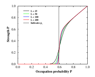
Fundamental results in percolation theory are all based on the assumption that the system sizes are infinite, as the spanning/percolating cluster is by definition an infinitely sized cluster that connects the entire system (e.g. end-to-end). However, in reality or at least in simulations, one is often dealing with finite systems, where all percolation related transitions are smeared out. So in order to determine the percolation threshold, one performs a finite size scaling analysis, where for instance the percolation strength (or probability) is computed as a function of occupation probability and repeats this for a range system sizes. Then, it is expected that if the studied systems have been large enough their curves will cross at a common point, which can be taken as an accurate estimate of the threshold in the limit of infinite system sizes.

These systems could be:

• Site or bond percolation: e.g., in 2D where a grid (often a lattice) is chosen where sites (or bonds) are occupied with a fixed probability $p.$ Two or more of such occupied sites that happen to be neighbours are then deemed to be a cluster. Then by computing the average of the maximum cluster size normalized by the number of sites as a function of $p,$ and repeated for various grid sizes $L,$ one can estimate the percolation threshold $p_c$ as their intersection point (example).
• As an example of a widely different system: suppose a suspension of spheres or cylinder-like objects in a 3D box. Then similarly, pairs of connected particles form clusters. These clusters grow in size with either increasing connectivity range or increasing density/volume-fraction. Therefore, in order to estimate the threshold in terms of the two aforementioned quantities, one computes the percolation probability as a function of them and across varying system sizes (box sizes here) and considers the so-obtained intersection as a the threshold. (example)

Example taken from these lecture notes:

Clearly, these systems have quite different details, but the fact that the same estimation method for determining $p_c$ is expected to hold generally, is unclear to me. I understand that if we take the comparison of system size $L$ and the correlation length $\xi,$ then there are two important regimes:

• $L\gg \xi:$ the relevant length scale remains the correlation length and we expect the known scaling laws for infinite systems to hold, namely $\xi \propto |p-p_c|^{-\nu}$ and the average cluster size $S\propto |p-p_c|^{-\gamma}.$ In this regime (corresponding to $p$ much larger than $p_c$), everything scales with $\xi,$ i.e., independent of system size $L.$

• But when $p$ approaches $p_c$ from the left, finite size effects are visible as the percolation probability, strength or average cluster size scales with $L.$

• Therefore, there is a crossover from the dependence on $L$ to $\xi$ when going from $p<p_c$ to $p>p_c.$

Questions:

1. Why this crossover suggests/implies that there should be a common intersection point for the curves of varying system sizes? Is this really expected to be the case irrespective of the details of the system (such as earlier examples)? Since in some cases, there may be additional relevant length scales, e.g. in the case of spheres or cylinders, we have not only $L$ (box size), but also the particles diameter (or aspect ratio) and the relative aspect ratio of the formed clusters with of the containing box. How can one rigorously assess all these length scales w.r.t to $L$ in order to make sure the systems are large enough and the curves will in fact intersect at same point?

2. How does one judge the system is large enough? Are there methods that allow us to test whether for a given system the method of intersecting curves of different $L$ is going to be valid? Because how we define $\xi$ in general may change from system to system.

tdlr: My attempt is to simply understand why this method works for estimating $p_c$ of so many widely different systems and what implies the intersection point, or at least how can we judge if it is going to work for a chosen problem. In many works, one often read "if the systems are large enough..." but I don't understand how large is supposed to be large enough.

Answer 1

The finite size scaling analysis is described in Appendix B of Thermal metal-insulator transition in a helical topological superconductor. This is for a different type of phase transition (metal-insulator instead of percolation), but the method of analysis is analogous.

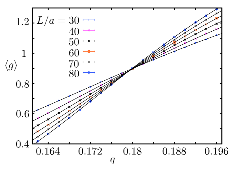
In summary, you have a quantity $g$ that depends on system size $L$ through a powerlaw function $F(u_0L^{1/\nu},u_1L^y)$, with exponents $1/\nu>0$ and $y<0$. In the large-$L$ limit only the $L^{1/\nu}$ term matters, that is the "scaling law" and $\nu$ is called the critical exponent. The $L^{y}$ term is the leading order correction to scaling. You perform a Taylor expansion of $F$ in powers of $u_0$ and $u_1$, up to some order $N_0$ and $N_1$, respectively. Then you fit the data to that functional form, with the coefficients of the Taylor expansion as the fit parameters. The result converges to something like the plot below (from the cited paper), and allows you to extract both the critical exponent $\nu$ as well as the critical point.

To answer specifically the first question: the functional form of $F$ is chosen such that there is a common intersection point by construction. If you fail to achieve a good fit, it indicates that the system has more than a single relevant scaling variable in the large-$L$ limit. That is certainly possible, but the physics of many phase transitions it that indeed, single-parameter scaling applies. So all microscopic parameters become irrelevant at the transition point, because of a diverging correlation length.

To answer the second question: the finite-size corrections to scaling are included in the fit, and you add higher and higher order terms until you reach a chi-squared value per degree of freedom of unity.