An experiment on random matrices

Question

A bit unsure if my use/mention of proprietary software might be inappropriate or even frowned upon here. If this is the case, or if this kind of experimental question is not welcome, please let me know and I'll remove it quickly.

I was experimenting on the distribution of eigenvalues of random matrices via the following Mathematica code

dim = 301;
decomplex = {z_Complex -> {Re[z], Im[z]}, A_Real -> {A, 0}}; b = 
 Eigenvalues[
   SparseArray[{i_, i_} -> 1, {dim, dim}] + 
    Table[RandomReal[{-.9, 1.}], {i, 1, dim}, {j, 1, dim}]] /. decomplex;
ListPlot[b, PlotStyle -> PointSize[0.015], AspectRatio -> Automatic]

This simply draws (or should draw) a picture of the complex eigenvalues of a 301 x 301 matrix, with entries uniformly distributed in the real interval [-0.9, 1]. If you try the code you will notice a disk of random eigenvalues, which is expected, plus a single positive eigenvalue at some distance of the disk. Decreasing the lower bound on the entries to -1 makes this phenomenon disappear, while increasing the lower bound makes it more evident.

Question: is this an artifact, a real phenomenon, or maybe even a well known and simple to explain phenomenon?

Answer 1

The distribution of the bulk of the spectrum is an example of the circular law. For the model you selected (where each entry is uniformly chosen at random from an interval), the law was first proven by Bai (at least in the case where the entries are normalised to have mean zero), building upon previous work of Girko; the non-central case (non-zero mean) was recently established by Chafai.

The non-central case is a rank one perturbation of the central case (by the matrix whose entries are all equal to the mean) and should therefore cause one exceptional eigenvalue.
(In the central case it can be shown that the spectral radius is close to the radius of the disk, so there are basically no exceptional eigenvalues.) If the mean of each entry is $\mu$, then the rank one perturbation has an eigenvalue at $\mu n$, so one expects the exceptional eigenvalue to linger near this number. In your case, $\mu = 0.05$ and $n = 301$, so the exceptional eigenvalue should linger near $15.05$.

There is a paper of Silverstein which makes the above heuristics precise; see also the earlier work of Andrew.

There is quite a bit of recent literature on the circular law, see for instance this survey by Van Vu and myself, or my lecture notes on this topic.

Answer 2

It looks like Joseph O'Rourke has beaten me, but I've generated a bit more data than he has:

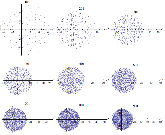
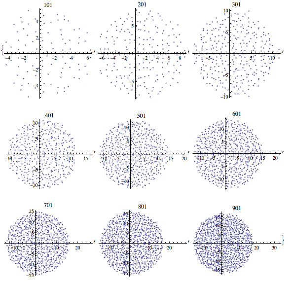
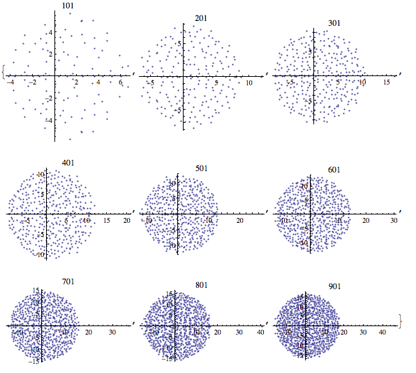
Let $l$ be the lower bound so that the non-diagonal entries are uniformly distributed between $l$ and 1 and the diagonal entries are distributed between $l+1$ and 2. Note that Piero's original characterization of his code was inaccurate, but I just used his code to generate the figures below.

Here is a grid of eigenvalues of such $N$ by $N$ matrices with $l=-.9$ (plots are labeled by $N$):

Here's the picture with $l=-.87$:

Here's the picture with $l=-.93$:

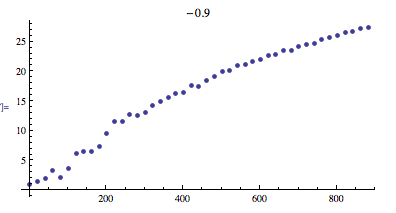
And here's a picture of the absolute value of the largest eigenvalue of the matrix as a function of $N$ (now the label is $l$):

Edit based on Helge's comment: Here's a picture of $\max_{1\leq j \leq N} \sum_{n=1}^{N} u_j^N(n)$ as a function of $N$ (the $u_j^N$ are normalized eigenvectors) with $l=-0.9$:

And here's a picture of the further normalized version $\max_{1\leq j \leq N} \frac{1}{\sqrt{N}}\sum_{n=1}^{N} u_j^N(n)$:

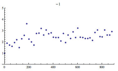
Edit 2: In response to Helge's comment asking for a plot of $\max_{1\leq j \leq N} \sum_{n=1}^{N} u_j^N(n)$ when $l=-1$:

Answer 3

Here is the output from Piero's posted code:

Answer 4

Why is your dimension 301? Does this phenomenon appear for dimension 300? Which seems like a more natural number to try this computation at.

Now as simple thought, about rescaling your matrix. If $A$ is matrix, whose entries are uniformly distributed in $[a,b]$ then $\lambda A$ is a matrix, whose entries are uniformly distributed in $[\lambda a , \lambda b]$. Define $$ B = \begin{pmatrix} 1 & \dots & 1 \\\ \vdots & \ddots & \vdots \\\ 1 & \dots & 1 \end{pmatrix}, $$ the matrix containing all ones. Then the entries of $A + \mu B$ have distribution $[a + \mu, b + \mu]$. Since, you know everything about $B$, that is it has the eigenvalue $$ v =\begin{pmatrix} 1 \\\ \vdots \\\ 1 \end{pmatrix} $$ to the eigenvalue $n$ (if $B$ is a $n\times n$ matrix). You see that you expect the eigenvalues $\lambda_j$ to the eigenvector $u_j$ of $A$ to be moved to $$ \lambda_j + \mu n \cdot \langle u_j, v\rangle $$ by first order perturbation theory. I think if $301$ is really a special choice, the conclusion is that in this case one of the eigenvectors of the random matrix is almost parallel to $v$.