3
$\begingroup$

I have a question about a reflecting Brownian motion and its boundary local time.

Bass and Hsu studied the existence of Reflecting Brownian motion and boundary local time on a bounded Lipschitz domain in 1991. Although I don't state the definition of boundary local time here, I will briefly explain what it is. Roughly speaking, boundary local time $\{L_{t}\}$ is an additive functional on a probability space and satisfies the following the equation: \begin{align*} L_{t}=\int_{0}^{t}1_{\left\{X_{s} \in \partial D \right\}}\,dL_{s}, \end{align*} where $\{X_{t}\}$ is a Reflecting Brownian motion on $\bar{D}$ (closure of a bounded Lipschitz domain $D$). That is, $L_t$ increases only when $X_t \in \partial D$.

Question

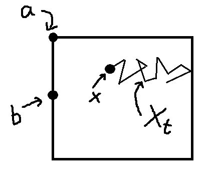
Let $D$ be a rectangle like as the follwong picture. Even in this case, we can define reflecting Brownian motion $(X_t,P_x)$ starting from $x \in \bar{D}$ and boundary local time $\{L_{t}\}$.

I am interested in the quantity $ P_{x}(L_t>M), $ where $M$ is a positive constant.

I think $P_{a}(L_t >M) \ge P_{b}(L_t >M)$, where $a,b$ are boundary points in the following picture. But I don't know how to prove this inequality. If you know related studies, please let me know.

enter image description here

ADD

In this question, $\{X_{t}\}$ is the Markov process generated by the following Dirichlet form on $L^{2}(\bar{D})$: \begin{align*} \mathcal{E}(f,g)=\frac{1}{2}\int_{D}(\nabla f, \nabla g)\,dx,\quad f,g \in H^1(D), \end{align*} where $H^{1}(D)$ is the Sobolev space on $D$ with Neumann boundary condition. $\{L_{t}\}$ is the positive continuous additive functional associated with the surface measure on $\partial D$. To be more precise, $\{L_t\}$ and $\sigma$ are in the Revuz correspondence. Futheremore, $X_{t}$ has the following Skorohod representation: \begin{align*} X_t=X_0+B_t+\frac{1}{2}\int_{0}^{t}n(X_s)\,dL_s, \end{align*} where $\{B_t\}$ is the $d$-dimensional Brownian motion and $n$ is the unit inward normal vector to $\partial D$.

$\endgroup$
6
  • $\begingroup$ Can you please specify the reflection (or constraint) directions? Otherwise your description of the reflecting Brownian motion is a bit incomplete. $\endgroup$ Sep 1, 2016 at 18:55
  • $\begingroup$ Thank you for pointing it out. $X_t$ is a Brownian motion in $D$ with normal reflection at the boundary. $\endgroup$
    – sharpe
    Sep 2, 2016 at 7:14
  • 1
    $\begingroup$ Is this process independent 1 d processes reflected at an upper & lower boundary? $\endgroup$
    – user83457
    Sep 2, 2016 at 10:33
  • $\begingroup$ In the Neumann case, the components of the RBM are completely decoupled. Therefore, I do not understand the point of the second component. Please clarify. $\endgroup$ Sep 2, 2016 at 12:32
  • $\begingroup$ For the moment, I tried to clarify my question. $\endgroup$
    – sharpe
    Sep 2, 2016 at 14:06

1 Answer 1

2
$\begingroup$

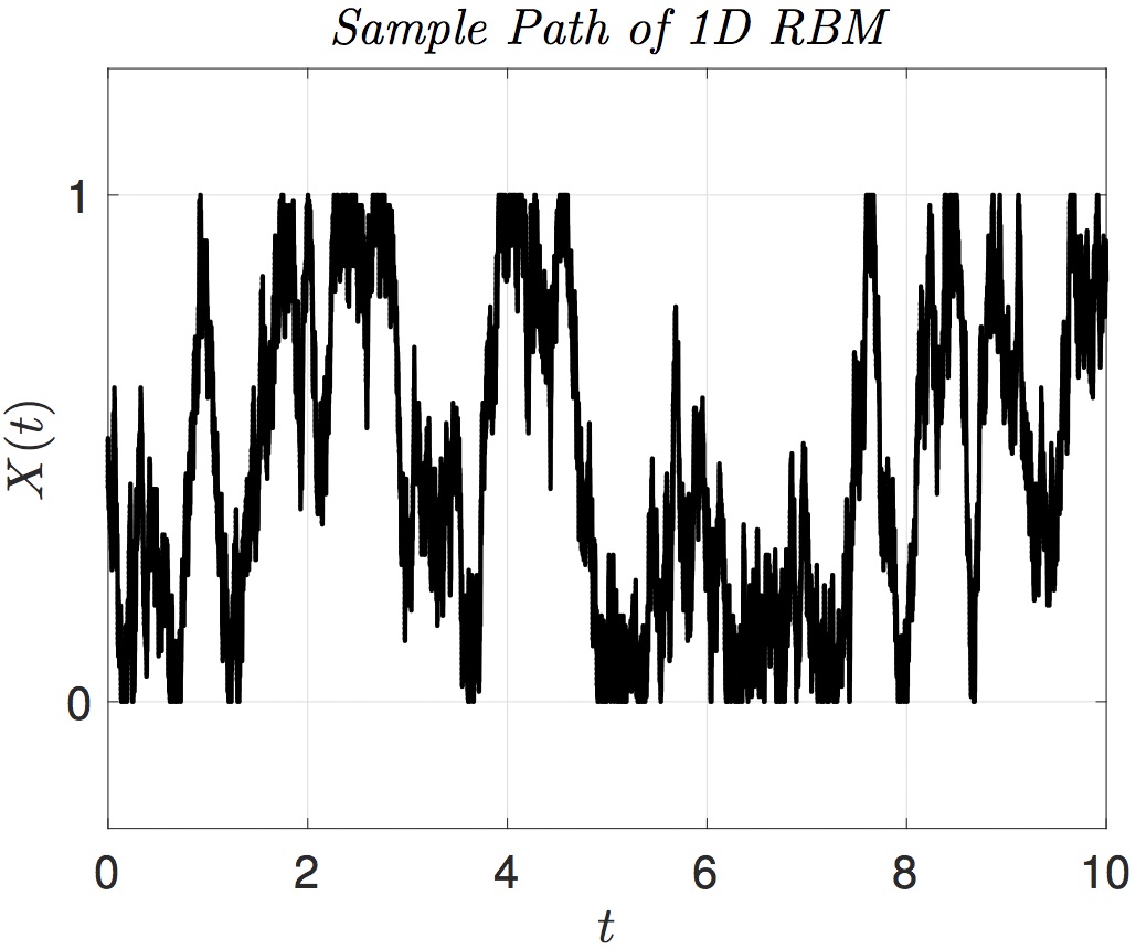
Since the components of the given planar RBM are uncoupled, it suffices to consider a scalar RBM $X$ on the spatial interval $[0,1]$. Here is a sample path of this process on the temporal interval $[0,10]$.

sample path

I will approach local time via the occupation time $$ \int_0^t 1_{[0, \epsilon]}(X(s)) ds $$ which gives the (random) amount of time the process spends in an $\epsilon$ neighborhood of zero during the interval $[0, t]$. This is a fairly complicated random variable, since it depends on the entire path of the RBM. However, its expected value is analytically available. Let $$ u^{\epsilon}(t,x) = \mathbb{E}_x \int_0^t 1_{[0, \epsilon]}(X(s)) ds \;. $$ Note that $u^{\epsilon}(t,x)$ satisfies an inhomogeneous initial boundary value problem: $$ \partial_t u^{\epsilon}(t,x) = \frac{1}{2} \partial_{xx} u^{\epsilon}(t,x) + 1_{[0, \epsilon]}(x) \quad \forall x \in [0,1] \;, \forall t \ge 0 \;, $$ with initial data $u(0,x)=0$ and pure Neumann boundary conditions $\partial_x u(t,0) = \partial_x u(t,0) = 0$. By expanding the solution and the inhomogeneity in terms of the eigenfunctions of the second derivative operator $\{ e_j(x) \}$ on $[0,1]$ with pure Neumann boundary conditions at $0$ and $1$, one obtains the following explicit solution: $$ u^{\epsilon}(t,x) = \epsilon t + 2^{3/2} \sum_{j \ge 2} \left( 1- \exp\left( \frac{t}{2} (j-1)^2 \pi^2 \right) \right) \frac{\sin( (j-1) \pi \epsilon)}{(j-1)^3 \pi^3} e_{j}(x) $$
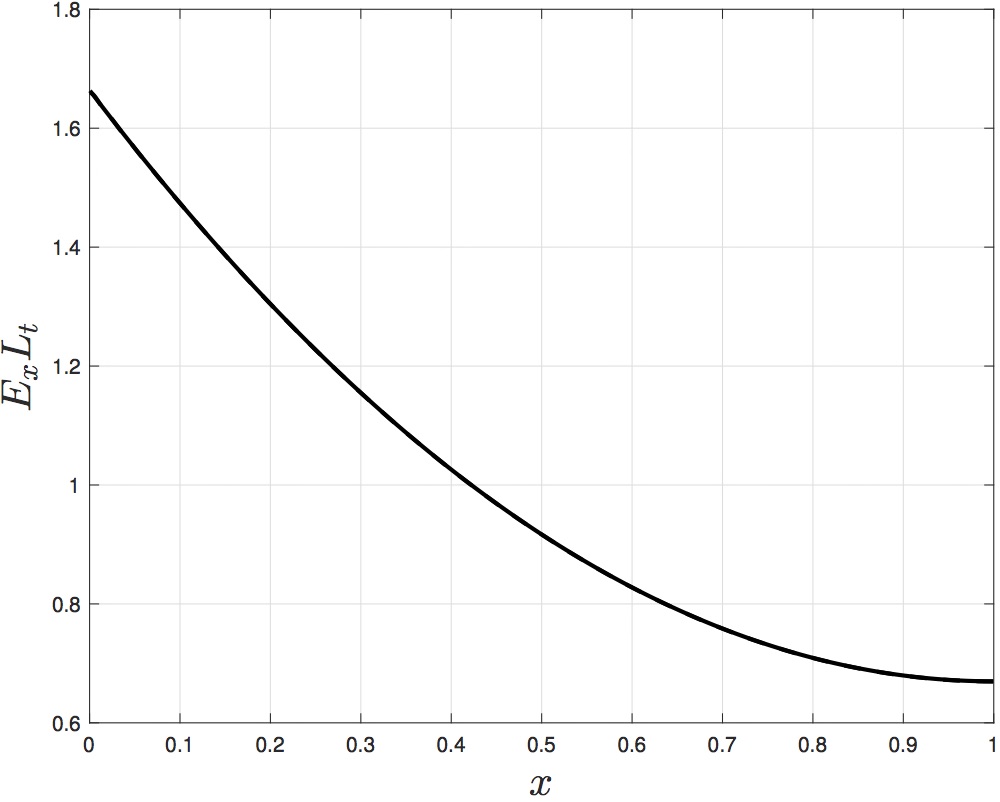
The following figure plots the behavior of $E_x L_t := \lim_{\epsilon \downarrow 0} \frac{u^{\epsilon}(t,x)}{\epsilon}$ as a function of the initial condition of the RBM $X(0)=x$ with $t=1$. As expected, this quantity decreases with distance from zero. (Since $t=1$, I find it curious that this quantity is greater than unity.)

local time

To answer the question, just view $x$ in this figure as the vertical component of the cartoon given in the question. As we already said, what happens in the horizontal component can be treated separately.

ADD

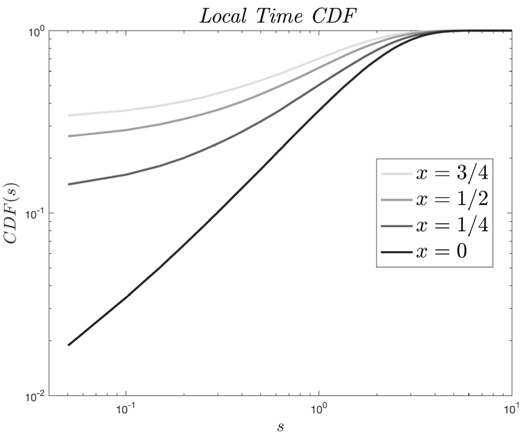
By using Monte-Carlo simulation, it is straightforward to obtain even more detail about the random variable $L_t^{\epsilon} = \epsilon^{-1} \int_0^t 1_{[0, \epsilon]}(X(s)) ds$. Here are graphs of the cumulative distribution function $CDF(s)=\mathbb{P}_x(L_t^{\epsilon} \le s)$ with $t=1$, for the initial conditions $X(0)=x$ indicated in the figure legend, and for $\epsilon$ sufficiently small. Logarithmic scaling is adopted to make it easier to compare the CDFs.

local time cdf

$\endgroup$
3
  • 1
    $\begingroup$ Thank you for your kind answer. But I am interested in boundary local time. In $1$D case, boundary local time $L_t$ may be characterized by $E_{x}[L_t]=\lim_{\epsilon \to 0}u_{\epsilon}(t,x)/\epsilon$, $u_{\epsilon}(t,x)=\int_{0}^{t}1_{[0,\epsilon]}(X_s)\,ds+\int_{0}^{t}1_{[1-\epsilon,1]}(X_s)$. Futhermore, $E_{0}[L_t]=E_{1}[L_t]$ should hold and $E_{x}[L_t] \ge E_{1/2}[L_t]$ for every $x \in[0,1]$. In this case, can we show $P_{x}(L_t \ge \alpha ) \ge P_{1/2}(L_t \ge \alpha)$? $\endgroup$
    – sharpe
    Sep 3, 2016 at 8:57
  • $\begingroup$ Motivated by your question, I added a bit more detail to my answer. $\endgroup$ Sep 3, 2016 at 18:55
  • $\begingroup$ Thank you for your answer. I think it may be difficult to show $P_x(L_t \ge \alpha) \ge P_{1/2}(L_t \ge \alpha)$. $\endgroup$
    – sharpe
    Sep 3, 2016 at 20:22

Your Answer

By clicking “Post Your Answer”, you agree to our terms of service and acknowledge you have read our privacy policy.

Not the answer you're looking for? Browse other questions tagged or ask your own question.