Distribution of distances in permutations

Question

Let's consider all possible permutations of N numbers. Suppose for each permutation we calculate the sum of absolute differences between consecutive elements. Thus, for (1,2,3) one would have abs(1-2)+abs(2-3)=2. Is it possible to obtain a distribution of such sums for given N? For instance, for N=3 one would have 3!=6 permutations and possible sums as 2 and 3. The number of sums of 2 is 2 and for 3 it's equal 4.

Answer 1

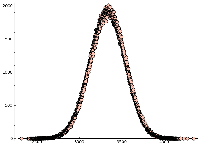
Here is a histogram for length 100. It seems to be normally distributed around $100^2 / 3$, which should put you on the scent, in spite of a complete absence of proof (see edit below).

This is not at all surprising, since if $x$ and $y$ are drawn uniformly at random from the interval $[0,1]$, the expected value of $|x-y|$ is $$ \int_{x=0}^1 \left(\frac{x^2}{2} + \frac{(1-x)^2}{2}\right) = \frac 13. $$ Maybe turning this fact into a proof is very straightforward; maybe it is tricky.

Edit: I should note that the expected value of $(n^2-1)/3$ actually is very easy to prove; it is just the distribution that might be tricky.

One way to generate a random permutation $\pi$ is to choose $n$ reals $r(i)$ uniformly at random from $[0,1]$. Now, what is the expected value of $|\pi(i) - \pi(i+1)|$? It is simply the expected number of $r(j)$ between $r(i)$ and $r(i+1)$, plus one. Because the expected difference between $r(i)$ and $r(i+1)$ is $1/3$, this is $1+(n-2)/3$, or $(n+1)/3$. Since we compute this for $n-1$ consecutive pairs, linearity of expectation tells us that the expected sum is $(n-1)(n+1)/3$, or $(n^2-1)/3$.

Answer 2

Andrew King pointed out that $E[X]$ is $(n^2-1)/3$.

So, to calculate the variance $E[X^2] - E[X]^2$ we need to find $E[X^2]$.

Let $\delta(i) = |\pi(i+1)-\pi(i)|$, so $X = \sum_{i=1}^{N-1} \delta(i)$.

$$\begin{eqnarray}X^2 &=& \bigg(\sum_{i=1}^{N-1} \delta(i)\bigg)^2 \newline &=& \sum_{i=1}^{N-1} \delta(i)^2 + 2 \sum_{i=1}^{N-2} \delta(i)\delta(i+1) + \sum_{|i-j|\gt 1} \delta(i)\delta(j) \end{eqnarray}$$

We can compute the expected values of each of these terms to find $E[X^2]$. By symmetry, we only need to find $(N-1)E[\delta(1)^2]$, $2(N-2)E[\delta(1)\delta(2)]$, and $((N-2)(N-3))E[\delta(1)\delta(3)].$

$$\begin{eqnarray}E[\delta(1)^2] &=& \frac{1}{N(N-1)} ~\sum_{a,b} (b-a)^2 \newline &=& \frac{1}{N(N-1)} \frac{N^4-N^2}{6} \newline &=&\frac{n^2+n}{6}\end{eqnarray}$$

I used Mathematica for the sums.

$$\begin{eqnarray} E[\delta(1)\delta(2)] &=& \frac{1}{N(N-1)(N-2)} \sum_{a,b,c~ \text{distinct}} |b-a||c-b| \newline &=& \frac{1}{N(N-1)(N-2)}\bigg(\sum_{a,b,c} |b-a||c-b| - \sum_{a,b,c | a=c} (b-a)^2 \bigg) \newline &=& \frac{1}{N(N-1)(N-2)} \bigg( \frac{7N^5 - 15N^3 - 8N}{60} - \frac{N^4-N^2}{6} \bigg)\newline &=& \frac{7N^2+11N+4}{60}\end{eqnarray}$$

The diagonal terms evaluate to $0$ or resemble the first sum.

$$\begin{eqnarray} E[\delta(1)\delta(3)] &=& \frac{1}{N(N-1)(N-2)(N-3)} \sum_{a,b,c,d ~ \text{distinct}} |b-a||d-c|\newline &=& \frac{1}{N(N-1)(N-2)(N-3)} \bigg( \sum_{a,b,c,d} |b-a||d-c| \newline & & - 4 \sum_{a,b,c,d | b=d} |b-a||c-b| + 2 \sum_{a,b,c,d|a=c,b=d} (b-a)^2 \bigg) \newline &=& \frac{1}{N(N-1)(N-2)(N-3)} \bigg( \frac{N^6-2N^4 + N^2}{9} \newline & & - 4\frac{7N^5-10N^4-15N^3+10N^2+8N}{60}+ 2 \frac{N^4-N^2}{6} \bigg) \newline &=& \frac{5N^5 - 21 N^4 + 35N^3+45N^2-40N -24}{45(N-1)(N-2)(N-3)} \newline &=& \frac{5N^4-16N^3+19N^2+64N+24}{45(N-2)(N-3)}\end{eqnarray}$$

If I calculated correctly, then

$$\begin{eqnarray}E[X^2] &= &\frac{N^3-N}{6} + \frac{7N^3-3N^2-18N-8}{30} \newline & & + \frac{5N^4-16N^3+19N^2+64N+24}{45} \newline &=& \frac{10N^4+4N^3+29N^2+59N+24}{90}\end{eqnarray}$$

$$\begin{eqnarray}\text{Var}[X] &=& E[X^2] -E[X]^2 \newline &=& \frac{4N^3+49N^2+59N+14}{90} \end{eqnarray}$$

For $N=100$, the standard deviation is $\sqrt\frac{249773}{5}=223.505$.

I believe a similar (but simpler) technique can be used to approximate higher moments of $X$. The dominant term is where no differences are adjacent, and the moments should be approximately the same as for random functions to $\lbrace 1, ..., n \rbrace$ instead of permutations. I think the method of moments would allow one to prove that the distribution is asymptotically normal.