Approximating Jordan curves

Question

I'd like to capture the intuitive notion that a Jordan curve $\gamma_2$ “follows” or “approximates” another Jordan curve $\gamma_1$, i.e. goes somehow “parallel” to it or “oscillates” around it.

Consider a differentiable Jordan curve $\gamma_1: [0,1] \rightarrow \mathbb{R}^2$ and its normals, seen as straight lines crossing the curve perpendicularly. Consider another Jordan curve $\gamma_2$ with the following properties:

1. Each normal of $\gamma_1$ crosses $\gamma_2$ at least once. I.e., for each normal $n(s_1)$ of $\gamma_1$ there is an $s_2$ such that the point $\gamma_2(s_2)$ lies on $n(s_1)$.

2. Furthermore when $s_1 < s_1'$ then there are unique $s_2 \le s_2'$ such that $\gamma_2(s_2)$ lies on $n(s_1)$ and $\gamma_2(s_2')$ lies on $n(s_1')$.

Do these conditions suffice to capture the notion described above? For which “pathological ” cases do they eventually fail? How then would they have to be adjusted to capture the notion?

Further questions:

1. Under which extra conditions does “$\gamma_2$ follows $\gamma_1$” imply that $\gamma_1$ follows $\gamma_2$?

2. When $\gamma_2$ follows $\gamma_1$, (how) can the area enclosed by $\gamma_1$ and $\gamma_2$ be calculated via the distance function $d(s_1) = |\gamma_1(s_1) - \gamma_2(s_2)|$
   ($s_2$ the unique parameter according to condition 2 above)?

(Let the area enclosed by $\gamma_1$ and $\gamma_2$ be the symmetric difference $X_1 \triangle X_2 = (X_1 \cup X_2) \setminus (X_1 \cap X_2)$ of the areas $X_1, X_2$ enclosed by $\gamma_1$ and $\gamma_2$.)

Answer 1

I would use the multiscale flat norm. (I am biased of course -- see: this paper on the multiscale flat norm)

You still need the minimization over rigid motions, but the flat norm is close to what you have come up with above. It works in any ambient dimension on surfaces of any co-dimension. It also does not require the surfaces you are comparing to be boundaries. The paper I wrote with Simon Morgan (linked to above) was primarily the observation that in the codimension one boundary case, the flat norm is computed by the $L^1$TV image operator. That has lots of nice consequences, like fast algorithms to do the calculations and a very useful (though simple) generalization of the classical flat norm.

The basic idea is explained carefully (and intuitively) in the paper, but I will also explain it very briefly here.

To find the distance between two k-dimensional currents $T_1$, $T_2$ (think of currents as surfaces with orientations), you can

1. decompose $T_1 - T_2$ into two pieces, $T_1 - T_2 = E + \partial S$, where $E$ is a k-current and $S$ is a k+1-current, so $\partial S$ is again a k-current,
2. charge yourself $M(E) + M(S)$ for the decomposition, where $M$ is the mass, measuring the k-volume of $E$ and the k+1-volume of $S$, and
3. minimize this cost over all k+1-currents $S$.
4. The result is the flat norm of $T_1 - T_2$, $\Bbb{F}(T_1-T_2)$.

Collecting all of this into one equation, the flat norm of a current T (we were choosing $T = T_1 - T_2$ above) is given by:

$\hspace{1in}\Bbb{F}(T) = \min_{\text{ k-currents }S} ( M(T-\partial S) + M(S)$)

---

Here is an image illustrating this for the case $k = 1$:

^(source)

For optimal $S$, $\Bbb{F}(T)$ is therefore the length of $T-\partial S$ plus the 2-dimensional area of $S$ (for the optimal $S$).

---

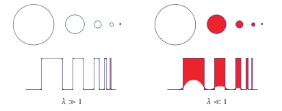
Finally, adding a parameter $\lambda$ permits us to controlling the tradeoff point between length and area. This gives us the $\color{blue}{\text{multiscale flat norm}}$:

$\hspace{1in}\Bbb{F}(T,\lambda) = \min_{\text{ k-currents }S} ( M(T-\partial S) + \lambda M(S)$)

If $\lambda$ is really big, we like length and try to avoid paying for area in $S$, if $\lambda$ is small then we prefer to replace cost of length with the cost of area whose boundary is used to cancel length. In the following image, for small $\lambda$'s we cancel all of the length cost in all but the largest circle:

^(source)

---

$\color{blue}{\text{A cool result: }}$ for minimizing decompositions, the mean curvature of $T-\partial S$ is bounded above by $\lambda$.