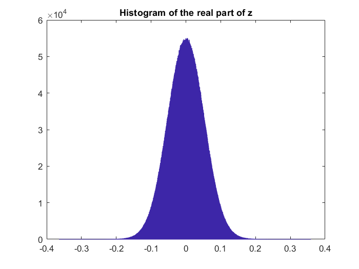
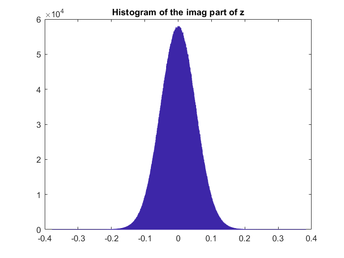
Let $n:=M$. Since you say "the denominator follows a Chi-square distribution with $2M$ degrees of freedom", it appears that you assume the $x_i$'s to be iid standard complex Gaussian; anyway, if you need $a>1$, then you can do a simple rescaling.
Thus, let us assume indeed that the $x_i$'s are iid standard complex Gaussian. It is then clear that the distribution of $z$ in $\mathbb C=\mathbb R^2$ is rotation invariant. So, it is enough to find the distribution of $|z|^2$, which is the same as that of
\begin{equation*}
R:=\frac X{(X+Y)^2},
\end{equation*}
where $X$ and $Y$ are independent random variables such that $X\sim\text{Gamma}(1,2)$ and $Y\sim\text{Gamma}(n-1,2)$.
Considering now the transformation from $(X,Y)$ to $(R,S)$ with $S:=X$ (say) and using the corresponding formula -- see e.g. formula (41) in Transformations,
we obtain the joint density of $(R,S)$, say $f_{R,S}$. Then the density of $R$ is given by the formula
\begin{equation*}
f_R(r)=\int_0^\infty f_{R,S}(r,s)\,ds.
\end{equation*}
Using in this integral the substitution $v=\sqrt{rs}$, we find
\begin{equation}
f_R(r)=\frac1{(n-2)!2^n r^{n+1}}\,\int_0^1 v^n(1-v)^{n-2}\exp\Big\{-\frac v{2r}\Big\}\,dv \tag{1}
\end{equation}
for $r>0$, with $f_R(r)=0$ for $r\le0$.
Using the binomial expansion for $(1-v)^{n-2}$ and then integrating by parts, we can express the latter integral as a finite sum (with the number of summands depending on $n$) of elementary functions.
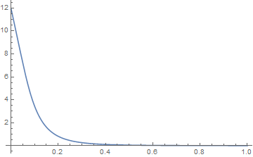
For instance, for $n=3$ and $r>0$
\begin{equation*}
f_R(r)=\exp\Big\{-\frac1{2r}\Big\}\left(\frac{1}{2 r^2}+96 r+\frac{6}{r}+36\right)-96 r+12;
\end{equation*}
here is the graph of this function:

However, by the dominated convergence theorem, the integral in (1) converges to $c_n:=\int_0^1 v^n(1-v)^{n-2}\,dv=n!(n-2)!/(2n-1)!$ as $r\to\infty$, and so, $f_R(r)\sim \frac{c_n}{(n-2)!2^n r^{n+1}}$ as $r\to\infty$. So, the tail of the distribution of $|z|^2$ is power-like, which shows that "the resulting distribution [of $z$]" is not Gaussian.
Addition in response to the modification of the OP's original question: There are many bell-shaped distributions, in addition to the family of Student $t_d$ distributions with $d$ degrees of freedom -- which includes the Cauchy distribution (for $d=1$) and, as a limit case (for $d=\infty$), the standard normal distribution.
Let $U$ denote the real part of $z$: $U:=\Re z$. You seem to be asking if the distribution of $U$ is $t_d$ for some $d\in(0,\infty]$. The answer to this is no, even if you allow rescaling of the distribution.
Indeed, from formula (1), using the Fubini theorem, it is easy to find all the moments of $|z|^2$:
\begin{equation*}
E|z|^{2m}=ER^m=\frac{m!(n-m-1)!}{2^m(n+m-1)!}
\end{equation*}
for $m=1,\dots,n-1$. So, the kurtosis of $|z|$ is
\begin{equation}
\frac{E|z|^4}{(E|z|^2)^2}=\frac{2n(n-1)}{(n+1)(n-2)}, \tag{2}
\end{equation}
for $n>2$.
On the other hand, if the distribution of $U=\Re z$ were $t_d$ for some $d\in(0,\infty]$, then
$|z|^2$ would equal $T_1^2+T_2^2$ in distribution, where $T,T_1,T_2$ are iid $t_d$, and so,
the kurtosis of $|z|$ would be
\begin{equation}
\frac{E(T_1^2+T_2^2)^2}{(ET_1^2+ET_2^2)^2}=\frac12+\frac12\,\frac{ET^4}{(ET^2)^2}=\frac{2d-5}{d-4}, \tag{3}
\end{equation}
for $d>4$.
On the other hand, the pdf $f_T(t)$ of $t_d$ is $\sim C_d t^{-d-1}$ (as $t\to\infty$), where $C_d$ does not depend on $t$. So, the pdf $f_{T^2}(u)$ is $\sim \frac12\,C_d u^{-d/2-1}$ (as $u\to\infty$). So, $f_{T_1^2+T_2^2}(u)\sim C_d u^{-d/2-1}$ (as $u\to\infty$). As mentioned above, $f_{|z|^2}(r)=f_R(r)\sim \frac{c_n}{(n-2)!2^n r^{n+1}}$ as $r\to\infty$.
So, if the distribution of $U=\Re z$ were $t_d$ for some $d\in(0,\infty]$, then the exponent $-d/2-1$ would be equal $-(n+1)$, so that $d=2n$ -- but then the kurtoses in (2) and (3) would be unequal, for any $n>2$.
Moreover, since the kurtosis is not affected by rescaling, the distribution of $U=\Re z$ cannot be $t_d$ for any $d\in(0,\infty]$ -- even if the distribution is rescaled by some positive real constant factor.
Addition in response to a comment by the OP: To find the pdf of $U=\Re z$, one can again use the referenced transformation technique. Indeed, without loss of generality, $U=\sqrt R\,C$, where $C:=\cos\Theta$ and $\Theta$ is a r.v. independent of $R$ and uniformly distributed in the interval $[0,2\pi]$ or, by symmetry, in $[0,\pi]$, so that for the pdf $f_C$ of $C$ one has $f_C(c)=\frac1\pi\,/\sqrt{1-c^2}$ for $-1<c<1$. Considering now the transformation from $(R,C)$ to $(U,W)$, where $U=\sqrt R\,C$ and $W=R$, we have the following rather complicated expression for the pdf of $U$:
\begin{equation*}
f_U(u)=\int_{u^2}^\infty \frac1{\pi\sqrt w}f_R(w)\frac{dw}{\sqrt{1-u^2/w}}
=\frac1\pi\,\int_{u^2}^\infty \frac{f_R(w)\,dw}{\sqrt{w-u^2}}
\end{equation*}
for all real $u$, where $f_R$ is given by (1).
Using the Fubini theorem and Mathematica for the calculation of the iterated double integral, we get
\begin{equation*}
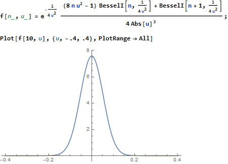
f_U(u)=\exp\Big\{{-\frac{1}{4 u^2}}\Big\} \,\frac{\left(8 n u^2-1\right) I_n\left(\frac{1}{4
u^2}\right)+I_{n+1}\left(\frac{1}{4 u^2}\right)}{4 |u|^3},
\end{equation*}
where $I_n(z)$ is the modified Bessel function of the first kind.
Below is the (bell-shaped) graph of $f_U=f_{\Re z}$ for $n=10$, which looks quite similar to your histogram. I am also including the corresponding Mathematica code:
