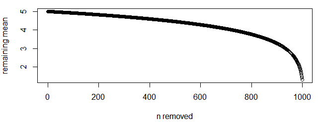
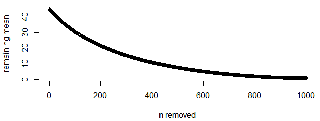
I doubt this is an easy analysis, as the result is going to be affected by the distribution used for $P(k)$. I doubt there is a general form, but empirically there may be a well-behaved example.
In any case, it seems possible to simulate what happens. There is no need to require the $P(k)$ to be integers so long as there probability $1$ that all the samples are positive.
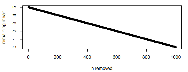
For example, if $P(k)$ has an exponential distribution with rate $\lambda$ i.e. mean $\frac1\lambda$, it seems from simulation that the expectation of the remaining empirical mean might be $\frac{N-n}{N}\frac1\lambda$ or close to that. As an illustration, here is a simulation using R, with $\lambda=\frac15$ and $N=10^3$ and averaging over $10^4$ cases:
set.seed(2024)
N <- 10^3
numbersims <- 10^4
remainingmean <- function(N){
  X <- rexp(N, 1/5) # distribution must take positive values
  Y <- sample(X, size=N, replace=FALSE, prob=X)
  return((sum(Y) - c(0,cumsum(Y)[-N])) / (N:1))
  }
sims <- replicate(numbersims, remainingmean(N))
plot(0:(N-1), rowMeans(sims), xlab="n removed", ylab="remaining mean")

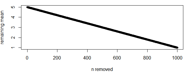
There is a distribution on the positive integers $\{1,2,3,\ldots\}$ similar to an exponential distribution, namely a suitable geometric distribution, and replacing the appropriate line in the code above with
X <- rgeom(N, 1/5) + 1 # distribution must take positive values
seems to produce a broadly similar chart (though necessarily heading towards $1$ rather than $0$):

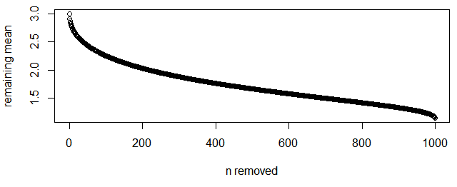
while a distribution with a lighter tail and a smaller variance, say a Poisson distribution plus $1$, declines more slowly initially
X <- rpois(N, 4) + 1 # distribution must take positive values

while a distribution with a heavier tail and greater variance, say the square of the geometric distribution, declines more quickly initially.
X <- (rgeom(N,1/5) + 1)^2 # distribution must take positive values

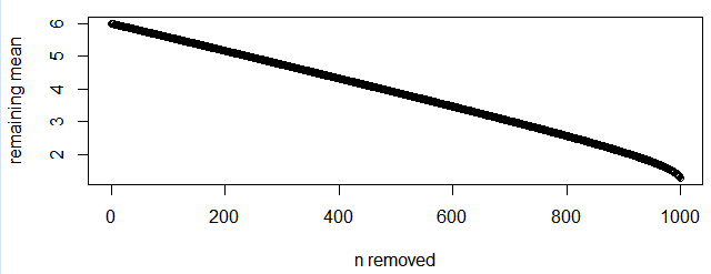
Apart from the unforeseen apparent linearity with an exponential distribution, this all seems intuitively reasonable, at least comparing one distribution with another. But it is not quite as simple as that: adding $1$ to the exponential distribution (so not changing the shape of the tail or the initial variance) keeps the close to linearity effect initially, but visually slightly deviates from it as $n$ reaches $N$ and so presumably deviates initially too but to a lesser effect.
X <- rexp(N, 1/5) + 1 # distribution must take positive values
