removed capitals from title
Source Link
YCor
  • 63.9k
  • 5
  • 187
  • 286

Upper bound for an Inverseinverse Laplace Transformtransform

Can anyone see how to get a tight upper bound for the function defined in terms of Inversethe inverse Laplace Transformtransform below? $$g_\text{sgd}(t)=\mathcal{L}^{-1}\left[\left(\frac{s}{2}+\frac{5 \sqrt{\frac{2}{3}} \sqrt{s}}{2 \tan ^{-1}\left(\frac{\sqrt{\frac{2}{3}}}{\sqrt{s}}\right)}\right)^{-1}\right].$$

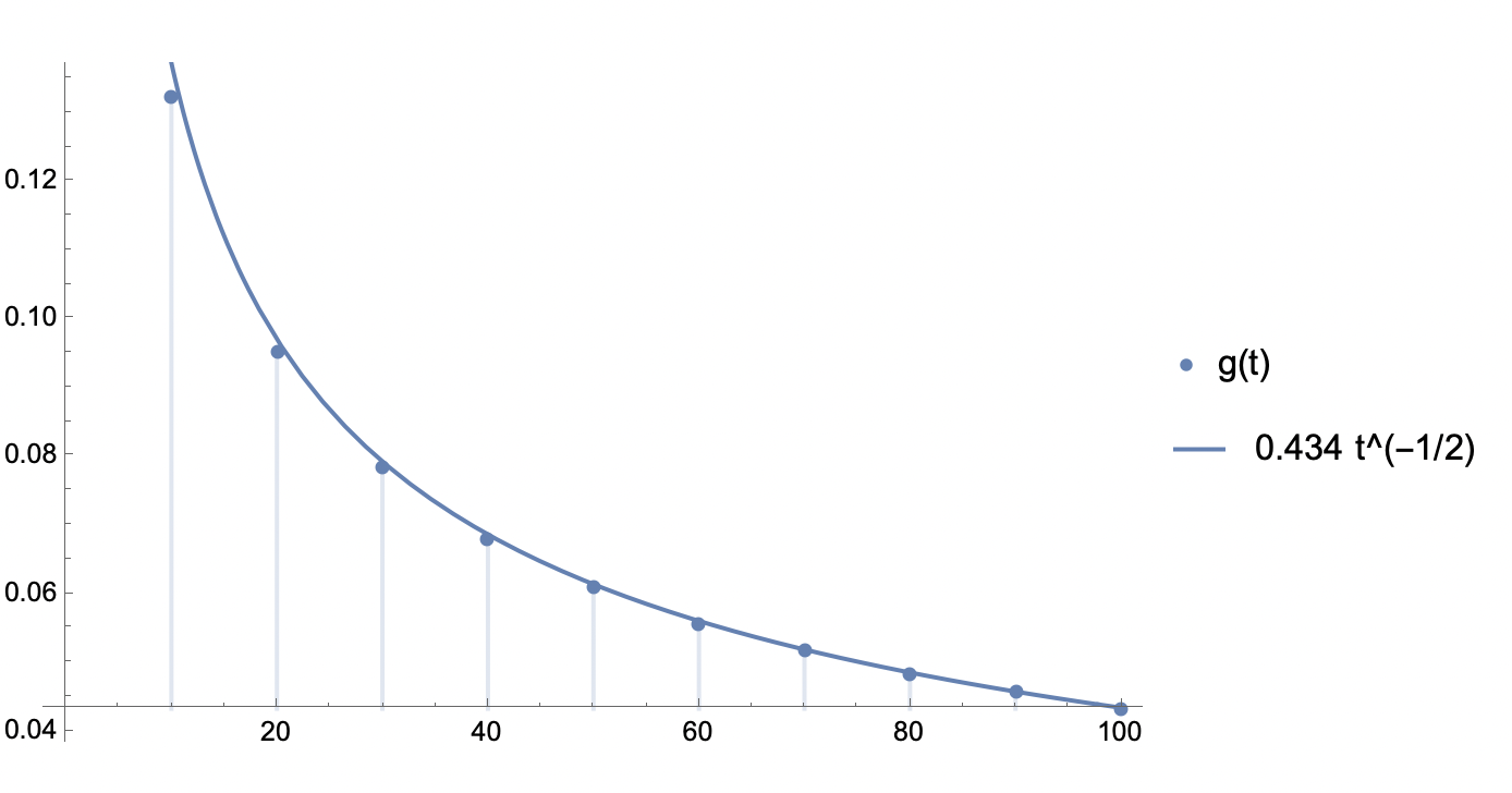
Dieter Kadelka's numerical simulation suggests $g_\text{sgd}(t)\approx 0.434 t^{-\frac{1}{2}}$, which appears to model this function very well...where does $O(t^{-\frac{1}{2}})$ form come from?

enter image description here Notebook

This function describes loss trajectory for stochastic gradient descent (SGD) on a linear least squares problem with covariance eigenvalues $1,\frac{1}{4},\frac{1}{9},\dotsc$. Expression comes when treating SGD as a continuous time problem which requires solving a particular differential equation

Upper bound for an Inverse Laplace Transform

Can anyone see how to get a tight upper bound for the function defined in terms of Inverse Laplace Transform below? $$g_\text{sgd}(t)=\mathcal{L}^{-1}\left[\left(\frac{s}{2}+\frac{5 \sqrt{\frac{2}{3}} \sqrt{s}}{2 \tan ^{-1}\left(\frac{\sqrt{\frac{2}{3}}}{\sqrt{s}}\right)}\right)^{-1}\right].$$

Dieter Kadelka's numerical simulation suggests $g_\text{sgd}(t)\approx 0.434 t^{-\frac{1}{2}}$, which appears to model this function very well...where does $O(t^{-\frac{1}{2}})$ form come from?

enter image description here Notebook

This function describes loss trajectory for stochastic gradient descent (SGD) on a linear least squares problem with covariance eigenvalues $1,\frac{1}{4},\frac{1}{9},\dotsc$. Expression comes when treating SGD as a continuous time problem which requires solving a particular differential equation
Upper bound for an inverse Laplace transform

Can anyone see how to get a tight upper bound for the function defined in terms of the inverse Laplace transform below? $$g_\text{sgd}(t)=\mathcal{L}^{-1}\left[\left(\frac{s}{2}+\frac{5 \sqrt{\frac{2}{3}} \sqrt{s}}{2 \tan ^{-1}\left(\frac{\sqrt{\frac{2}{3}}}{\sqrt{s}}\right)}\right)^{-1}\right].$$

Dieter Kadelka's numerical simulation suggests $g_\text{sgd}(t)\approx 0.434 t^{-\frac{1}{2}}$, which appears to model this function very well...where does $O(t^{-\frac{1}{2}})$ form come from?

enter image description here Notebook

This function describes loss trajectory for stochastic gradient descent (SGD) on a linear least squares problem with covariance eigenvalues $1,\frac{1}{4},\frac{1}{9},\dotsc$. Expression comes when treating SGD as a continuous time problem which requires solving a particular differential equation

edited body
Source Link

Can anyone see how to get a tight upper bound for the function defined in terms of Inverse Laplace Transform below? $$g_\text{sgd}(t)=\mathcal{L}^{-1}\left[\left(\frac{s}{2}+\frac{5 \sqrt{\frac{2}{3}} \sqrt{s}}{2 \tan ^{-1}\left(\frac{\sqrt{\frac{2}{3}}}{\sqrt{s}}\right)}\right)^{-1}\right].$$

Dieter Kadelka's numerical simulation suggests $g_\text{sgd}(t)\approx 0.434 t^{-\frac{1}{2}}$, which appears to model this function very well...where does $O(t^{-\frac{1}{2}})$ form come from?

enter image description here Notebook

TheseThis function describes loss trajectory for stochastic gradient descent (SGD) on a linear least squares problem with covariance eigenvalues $1,\frac{1}{4},\frac{1}{9},\dotsc$. Expression comes when treating SGD as a continuous time problem which requires solving a particular differential equation

Can anyone see how to get a tight upper bound for the function defined in terms of Inverse Laplace Transform below? $$g_\text{sgd}(t)=\mathcal{L}^{-1}\left[\left(\frac{s}{2}+\frac{5 \sqrt{\frac{2}{3}} \sqrt{s}}{2 \tan ^{-1}\left(\frac{\sqrt{\frac{2}{3}}}{\sqrt{s}}\right)}\right)^{-1}\right].$$

Dieter Kadelka's numerical simulation suggests $g_\text{sgd}(t)\approx 0.434 t^{-\frac{1}{2}}$, which appears to model this function very well...where does $O(t^{-\frac{1}{2}})$ form come from?

enter image description here Notebook

These function describes loss trajectory for stochastic gradient descent (SGD) on a linear least squares problem with covariance eigenvalues $1,\frac{1}{4},\frac{1}{9},\dotsc$. Expression comes when treating SGD as a continuous time problem which requires solving a particular differential equation

Can anyone see how to get a tight upper bound for the function defined in terms of Inverse Laplace Transform below? $$g_\text{sgd}(t)=\mathcal{L}^{-1}\left[\left(\frac{s}{2}+\frac{5 \sqrt{\frac{2}{3}} \sqrt{s}}{2 \tan ^{-1}\left(\frac{\sqrt{\frac{2}{3}}}{\sqrt{s}}\right)}\right)^{-1}\right].$$

Dieter Kadelka's numerical simulation suggests $g_\text{sgd}(t)\approx 0.434 t^{-\frac{1}{2}}$, which appears to model this function very well...where does $O(t^{-\frac{1}{2}})$ form come from?

enter image description here Notebook

This function describes loss trajectory for stochastic gradient descent (SGD) on a linear least squares problem with covariance eigenvalues $1,\frac{1}{4},\frac{1}{9},\dotsc$. Expression comes when treating SGD as a continuous time problem which requires solving a particular differential equation

added Dieter's Kadelka's simulation
Source Link

Can anyone see how to get a tight upper bound for the function defined in terms of Inverse Laplace Transform below? $$g_\text{sgd}(t)=\mathcal{L}^{-1}\left[\left(\frac{s}{2}+\frac{5 \sqrt{\frac{2}{3}} \sqrt{s}}{2 \tan ^{-1}\left(\frac{\sqrt{\frac{2}{3}}}{\sqrt{s}}\right)}\right)^{-1}\right].$$

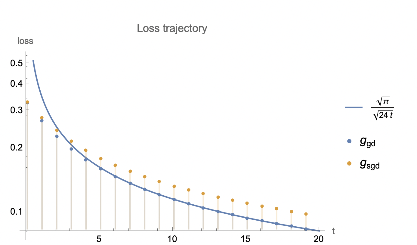
A closely related problem has a nice approximationDieter Kadelka's numerical simulation suggests $g_\text{sgd}(t)\approx 0.434 t^{-\frac{1}{2}}$, which I suspect is an upper bound, in plot below:

$$g_\text{gd}(t)=\mathcal{L}^{-1}\left[\frac{\pi -2 \tan ^{-1}\left(\sqrt{\frac{3}{2}} \sqrt{s}\right)}{2 \sqrt{6} \sqrt{s}}\right]\approx \frac{\sqrt{\pi }}{\sqrt{24 t}}.$$appears to model this function very well...where does $O(t^{-\frac{1}{2}})$ form come from?

enter image description hereenter image description here Notebook

These two functions describefunction describes loss trajectory for gradient descent (GD) and stochastic gradient descent (SGD) on a linear least squares problem with covariance eigenvalues $1,\frac{1}{4},\frac{1}{9},\dotsc$. Expressions comeExpression comes when treating GD/SGDSGD as a continuous time problem which requires solving a particular differential equation .

Working hypothesis is that $g_\text{sgd}(t)<\frac{\sqrt{\pi }}{\sqrt{12 t}}$.

Can anyone see how to get a tight upper bound for the function defined in terms of Inverse Laplace Transform below? $$g_\text{sgd}(t)=\mathcal{L}^{-1}\left[\left(\frac{s}{2}+\frac{5 \sqrt{\frac{2}{3}} \sqrt{s}}{2 \tan ^{-1}\left(\frac{\sqrt{\frac{2}{3}}}{\sqrt{s}}\right)}\right)^{-1}\right].$$

A closely related problem has a nice approximation, which I suspect is an upper bound, in plot below:

$$g_\text{gd}(t)=\mathcal{L}^{-1}\left[\frac{\pi -2 \tan ^{-1}\left(\sqrt{\frac{3}{2}} \sqrt{s}\right)}{2 \sqrt{6} \sqrt{s}}\right]\approx \frac{\sqrt{\pi }}{\sqrt{24 t}}.$$

enter image description here Notebook

These two functions describe loss trajectory for gradient descent (GD) and stochastic gradient descent (SGD) on a linear least squares problem with covariance eigenvalues $1,\frac{1}{4},\frac{1}{9},\dotsc$. Expressions come when treating GD/SGD as a continuous time problem which requires solving a particular differential equation .

Working hypothesis is that $g_\text{sgd}(t)<\frac{\sqrt{\pi }}{\sqrt{12 t}}$.

Can anyone see how to get a tight upper bound for the function defined in terms of Inverse Laplace Transform below? $$g_\text{sgd}(t)=\mathcal{L}^{-1}\left[\left(\frac{s}{2}+\frac{5 \sqrt{\frac{2}{3}} \sqrt{s}}{2 \tan ^{-1}\left(\frac{\sqrt{\frac{2}{3}}}{\sqrt{s}}\right)}\right)^{-1}\right].$$

Dieter Kadelka's numerical simulation suggests $g_\text{sgd}(t)\approx 0.434 t^{-\frac{1}{2}}$, which appears to model this function very well...where does $O(t^{-\frac{1}{2}})$ form come from?

enter image description here Notebook

These function describes loss trajectory for stochastic gradient descent (SGD) on a linear least squares problem with covariance eigenvalues $1,\frac{1}{4},\frac{1}{9},\dotsc$. Expression comes when treating SGD as a continuous time problem which requires solving a particular differential equation

Removing editorialising in title
Source Link
LSpice
  • 12.9k
  • 4
  • 45
  • 69
Loading
added 15 characters in body
Source Link
Loading
added 188 characters in body
Source Link
Loading
Source Link
Loading