added 359 characters in body
Source Link
Iosif Pinelis
  • 127.7k
  • 8
  • 107
  • 229

The DKW inequality can be stated as follows: \begin{equation} p_n(z):=P(\|S_n\|_\infty/\sqrt n>z)\le 2e^{-2z^2} \tag{1}\label{1} \end{equation}\begin{equation} p_n(z):=P(\|S_n\|_\infty>z)\le 2e^{-2z^2} \tag{1}\label{1} \end{equation} for $z>0$, where \begin{equation} S_n(t):=\sum_{i=1}^n Y_i(t),\quad Y_i(t):=1(X_i\le t)-t, \end{equation}\begin{equation} S_n(t):=\frac1{\sqrt n}\,\sum_{i=1}^n Y_i(t),\quad Y_i(t):=1(X_i\le t)-t, \end{equation} and the $X_i$'s are iid random variables (r.v.'s) each uniformly distributed on $[0,1]$.

You seem to say that your simulations appear to be suggesting that the constant factor $2$ in the exponent of $e^{-2z^2}$ in the bound in \eqref{1} must be replaced a constant factor that is about $2.5$ times worse than the constant factor $2$.


This suggestion is extremely unlikely to be true, given the very long and rich history of the DKW inequality. Apparently, this history begins with Kolmogorov and Smirnov, who showed that
\begin{equation} p_n(z)\to p(z):=2\sum_{k=1}^\infty(-1)^{k-1}e^{-2k^2z^2} \end{equation} for each $z>0$ as $n\to\infty$. Note that $p(z)\le 2e^{-2z^2}$ for all $z>0$ and $p(z)\sim 2e^{-2z^2}$ as $z\to\infty$. This strongly suggests that $2$ is the right (and the best possible) constant factor $2$ in the exponent of $e^{-2z^2}$ in \eqref{1}.

One may also note here the iid random functions $Y_i$ are zero-mean, each with the covariance function $[0,1]^2\ni(s,t)\mapsto EY_i(s)Y_i(t)=\min(s,t)-st$. So, the mean and covariance functions of each random function $Y_i$ are the same as those of the Brownian bridge. By an appropriate functional central limit theorem, it is at least plausible that the random function $S_n$ converges in an appropriate sense to a Gaussian process. Since the distribution of a Gaussian process is determined by its mean and covariance functions, it follows that the random function $S_n$ converges in an appropriate sense to a Brownian bridge $B^0$. So, it is likely that \begin{equation} p_n(z)\to P(\|B^0\|_\infty>z)=p(z); \tag{2}\label{2} \end{equation} concerning the latter equality, cf. e.g. this or this. Of course, \eqref{2} is, not only plausible, but true and well known. In particular, in view of (say) [Talangrand's Theorem 1.1] with $\mathcal F=\{1_{[0,t]}\colon t\in[0,1]\}$, $\|S_n-B^0\|_\infty$ converges to $0$ in probability as $n\to\infty$.

So, again, it is extremely unlikely that the DKW inequality is false. It is much more likely that the problem is with the software you were using and/or with your code, which I cannot read.


Below is an image of a Mathematica notebook confirming your inequality:

enter image description here

The DKW inequality can be stated as follows: \begin{equation} p_n(z):=P(\|S_n\|_\infty/\sqrt n>z)\le 2e^{-2z^2} \tag{1}\label{1} \end{equation} for $z>0$, where \begin{equation} S_n(t):=\sum_{i=1}^n Y_i(t),\quad Y_i(t):=1(X_i\le t)-t, \end{equation} and the $X_i$'s are iid random variables (r.v.'s) each uniformly distributed on $[0,1]$.

You seem to say that your simulations appear to be suggesting that the constant factor $2$ in the exponent of $e^{-2z^2}$ in the bound in \eqref{1} must be replaced a constant factor that is about $2.5$ times worse than the constant factor $2$.


This suggestion is extremely unlikely to be true, given the very long and rich history of the DKW inequality. Apparently, this history begins with Kolmogorov and Smirnov, who showed that
\begin{equation} p_n(z)\to p(z):=2\sum_{k=1}^\infty(-1)^{k-1}e^{-2k^2z^2} \end{equation} for each $z>0$ as $n\to\infty$. Note that $p(z)\le 2e^{-2z^2}$ for all $z>0$ and $p(z)\sim 2e^{-2z^2}$ as $z\to\infty$. This strongly suggests that $2$ is the right (and the best possible) constant factor $2$ in the exponent of $e^{-2z^2}$ in \eqref{1}.

One may also note here the iid random functions $Y_i$ are zero-mean, each with the covariance function $[0,1]^2\ni(s,t)\mapsto EY_i(s)Y_i(t)=\min(s,t)-st$. So, the mean and covariance functions of each random function $Y_i$ are the same as those of the Brownian bridge. By an appropriate functional central limit theorem, it is at least plausible that the random function $S_n$ converges in an appropriate sense to a Gaussian process. Since the distribution of a Gaussian process is determined by its mean and covariance functions, it follows that the random function $S_n$ converges in an appropriate sense to a Brownian bridge $B^0$. So, it is likely that \begin{equation} p_n(z)\to P(\|B^0\|_\infty>z)=p(z); \tag{2}\label{2} \end{equation} concerning the latter equality, cf. e.g. this or this. Of course, \eqref{2} is, not only plausible, but true and well known.

So, again, it is extremely unlikely that the DKW inequality is false. It is much more likely that the problem is with the software you were using and/or with your code, which I cannot read.


Below is an image of a Mathematica notebook confirming your inequality:
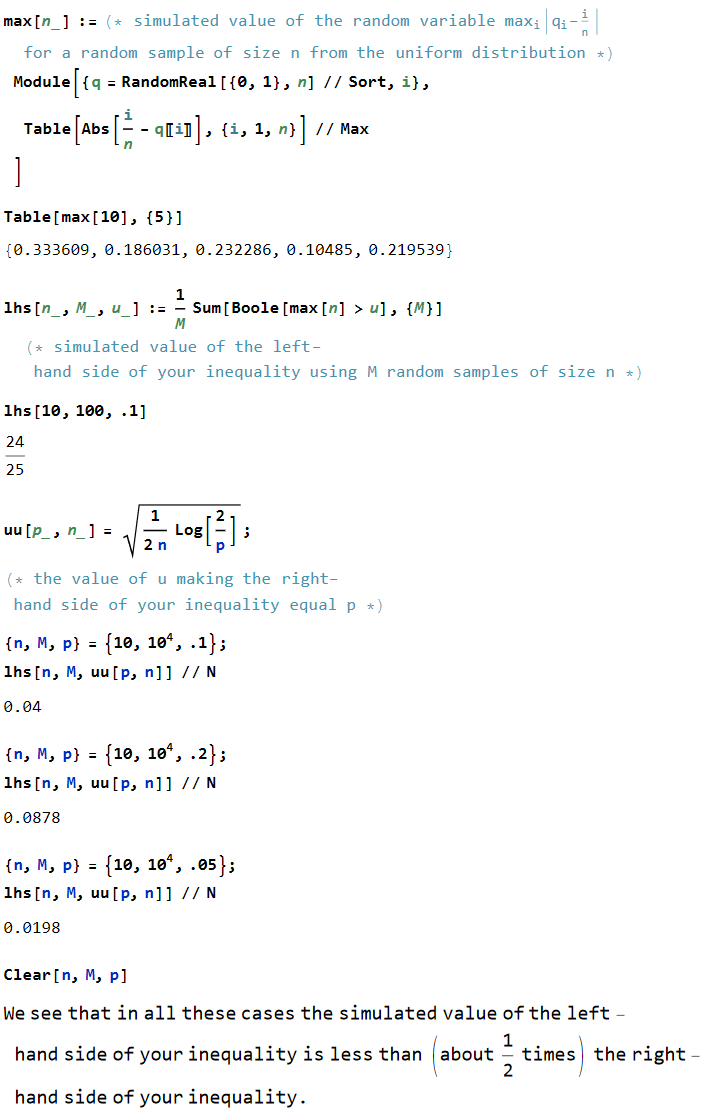
enter image description here

The DKW inequality can be stated as follows: \begin{equation} p_n(z):=P(\|S_n\|_\infty>z)\le 2e^{-2z^2} \tag{1}\label{1} \end{equation} for $z>0$, where \begin{equation} S_n(t):=\frac1{\sqrt n}\,\sum_{i=1}^n Y_i(t),\quad Y_i(t):=1(X_i\le t)-t, \end{equation} and the $X_i$'s are iid random variables (r.v.'s) each uniformly distributed on $[0,1]$.

You seem to say that your simulations appear to be suggesting that the constant factor $2$ in the exponent of $e^{-2z^2}$ in the bound in \eqref{1} must be replaced a constant factor that is about $2.5$ times worse than the constant factor $2$.


This suggestion is extremely unlikely to be true, given the very long and rich history of the DKW inequality. Apparently, this history begins with Kolmogorov and Smirnov, who showed that
\begin{equation} p_n(z)\to p(z):=2\sum_{k=1}^\infty(-1)^{k-1}e^{-2k^2z^2} \end{equation} for each $z>0$ as $n\to\infty$. Note that $p(z)\le 2e^{-2z^2}$ for all $z>0$ and $p(z)\sim 2e^{-2z^2}$ as $z\to\infty$. This strongly suggests that $2$ is the right (and the best possible) constant factor $2$ in the exponent of $e^{-2z^2}$ in \eqref{1}.

One may also note here the iid random functions $Y_i$ are zero-mean, each with the covariance function $[0,1]^2\ni(s,t)\mapsto EY_i(s)Y_i(t)=\min(s,t)-st$. So, the mean and covariance functions of each random function $Y_i$ are the same as those of the Brownian bridge. By an appropriate functional central limit theorem, it is at least plausible that the random function $S_n$ converges in an appropriate sense to a Gaussian process. Since the distribution of a Gaussian process is determined by its mean and covariance functions, it follows that the random function $S_n$ converges in an appropriate sense to a Brownian bridge $B^0$. So, it is likely that \begin{equation} p_n(z)\to P(\|B^0\|_\infty>z)=p(z); \tag{2}\label{2} \end{equation} concerning the latter equality, cf. e.g. this or this. Of course, \eqref{2} is, not only plausible, but true and well known. In particular, in view of (say) [Talangrand's Theorem 1.1] with $\mathcal F=\{1_{[0,t]}\colon t\in[0,1]\}$, $\|S_n-B^0\|_\infty$ converges to $0$ in probability as $n\to\infty$.

So, again, it is extremely unlikely that the DKW inequality is false. It is much more likely that the problem is with the software you were using and/or with your code, which I cannot read.


Below is an image of a Mathematica notebook confirming your inequality:
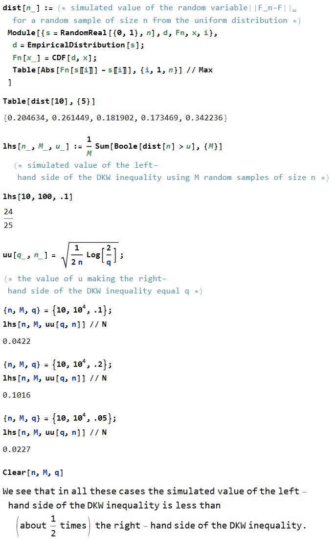
enter image description here

added 2572 characters in body
Source Link
Iosif Pinelis
  • 127.7k
  • 8
  • 107
  • 229

PerhapsThe DKW inequality can be stated as follows: \begin{equation} p_n(z):=P(\|S_n\|_\infty/\sqrt n>z)\le 2e^{-2z^2} \tag{1}\label{1} \end{equation} for $z>0$, where \begin{equation} S_n(t):=\sum_{i=1}^n Y_i(t),\quad Y_i(t):=1(X_i\le t)-t, \end{equation} and the $X_i$'s are iid random variables (r.v.'s) each uniformly distributed on $[0,1]$.

You seem to say that your simulations appear to be suggesting that the constant factor $2$ in the exponent of $e^{-2z^2}$ in the bound in \eqref{1} must be replaced a constant factor that is about $2.5$ times worse than the constant factor $2$.


This suggestion is extremely unlikely to be true, given the very long and rich history of the DKW inequality. Apparently, this history begins with Kolmogorov and Smirnov, who showed that
\begin{equation} p_n(z)\to p(z):=2\sum_{k=1}^\infty(-1)^{k-1}e^{-2k^2z^2} \end{equation} for each $z>0$ as $n\to\infty$. Note that $p(z)\le 2e^{-2z^2}$ for all $z>0$ and $p(z)\sim 2e^{-2z^2}$ as $z\to\infty$. This strongly suggests that $2$ is the right (and the best possible) constant factor $2$ in the exponent of $e^{-2z^2}$ in \eqref{1}.

One may also note here the iid random functions $Y_i$ are zero-mean, each with the covariance function $[0,1]^2\ni(s,t)\mapsto EY_i(s)Y_i(t)=\min(s,t)-st$. So, the mean and covariance functions of each random function $Y_i$ are the same as those of the Brownian bridge. By an appropriate functional central limit theorem, it is at least plausible that the random function $S_n$ converges in an appropriate sense to a Gaussian process. Since the distribution of a Gaussian process is determined by its mean and covariance functions, it follows that the random function $S_n$ converges in an appropriate sense to a Brownian bridge $B^0$. So, it is likely that \begin{equation} p_n(z)\to P(\|B^0\|_\infty>z)=p(z); \tag{2}\label{2} \end{equation} concerning the latter equality, cf. e.g. this or this. Of course, \eqref{2} is, not only plausible, but true and well known.

So, again, it is extremely unlikely that the DKW inequality is false. It is much more likely that the problem is with the software oryou were using and/or with your code, which I cannot read.


Below is an image of a Mathematica notebook confirming your inequality:

enter image description here

Perhaps the problem is with the software or your code, which I cannot read.

Below is an image of a Mathematica notebook confirming your inequality:

enter image description here

The DKW inequality can be stated as follows: \begin{equation} p_n(z):=P(\|S_n\|_\infty/\sqrt n>z)\le 2e^{-2z^2} \tag{1}\label{1} \end{equation} for $z>0$, where \begin{equation} S_n(t):=\sum_{i=1}^n Y_i(t),\quad Y_i(t):=1(X_i\le t)-t, \end{equation} and the $X_i$'s are iid random variables (r.v.'s) each uniformly distributed on $[0,1]$.

You seem to say that your simulations appear to be suggesting that the constant factor $2$ in the exponent of $e^{-2z^2}$ in the bound in \eqref{1} must be replaced a constant factor that is about $2.5$ times worse than the constant factor $2$.


This suggestion is extremely unlikely to be true, given the very long and rich history of the DKW inequality. Apparently, this history begins with Kolmogorov and Smirnov, who showed that
\begin{equation} p_n(z)\to p(z):=2\sum_{k=1}^\infty(-1)^{k-1}e^{-2k^2z^2} \end{equation} for each $z>0$ as $n\to\infty$. Note that $p(z)\le 2e^{-2z^2}$ for all $z>0$ and $p(z)\sim 2e^{-2z^2}$ as $z\to\infty$. This strongly suggests that $2$ is the right (and the best possible) constant factor $2$ in the exponent of $e^{-2z^2}$ in \eqref{1}.

One may also note here the iid random functions $Y_i$ are zero-mean, each with the covariance function $[0,1]^2\ni(s,t)\mapsto EY_i(s)Y_i(t)=\min(s,t)-st$. So, the mean and covariance functions of each random function $Y_i$ are the same as those of the Brownian bridge. By an appropriate functional central limit theorem, it is at least plausible that the random function $S_n$ converges in an appropriate sense to a Gaussian process. Since the distribution of a Gaussian process is determined by its mean and covariance functions, it follows that the random function $S_n$ converges in an appropriate sense to a Brownian bridge $B^0$. So, it is likely that \begin{equation} p_n(z)\to P(\|B^0\|_\infty>z)=p(z); \tag{2}\label{2} \end{equation} concerning the latter equality, cf. e.g. this or this. Of course, \eqref{2} is, not only plausible, but true and well known.

So, again, it is extremely unlikely that the DKW inequality is false. It is much more likely that the problem is with the software you were using and/or with your code, which I cannot read.


Below is an image of a Mathematica notebook confirming your inequality:

enter image description here

deleted 287 characters in body
Source Link
Iosif Pinelis
  • 127.7k
  • 8
  • 107
  • 229

The DKW inequality is $$P(\|F_n-F\|_\infty>u)\le2e^{-2nu^2}$$ for $u>0$, where $F$ isPerhaps the true cdf and $F_n$problem is with the empirical cdf.

Your inequality is different. It is something like this: $$P(\|F_n^{-1}-F^{-1}\|_\infty>u)\le2e^{-2nu^2}$$ for $u>0$. (It is unclear to me howsoftware or your (sample?) quantiles $q_i$ are defined;code, which I cannot read your code.)


Below is an image of a Mathematica notebook confirming the DKWyour inequality:

enter image description hereenter image description here

The DKW inequality is $$P(\|F_n-F\|_\infty>u)\le2e^{-2nu^2}$$ for $u>0$, where $F$ is the true cdf and $F_n$ is the empirical cdf.

Your inequality is different. It is something like this: $$P(\|F_n^{-1}-F^{-1}\|_\infty>u)\le2e^{-2nu^2}$$ for $u>0$. (It is unclear to me how your (sample?) quantiles $q_i$ are defined; I cannot read your code.)


Below is an image of a Mathematica notebook confirming the DKW inequality:

enter image description here

Perhaps the problem is with the software or your code, which I cannot read.

Below is an image of a Mathematica notebook confirming your inequality:

enter image description here

added 178 characters in body
Source Link
Iosif Pinelis
  • 127.7k
  • 8
  • 107
  • 229
Loading
added 58 characters in body
Source Link
Iosif Pinelis
  • 127.7k
  • 8
  • 107
  • 229
Loading
Source Link
Iosif Pinelis
  • 127.7k
  • 8
  • 107
  • 229
Loading